Performance Analysis for Coupled - Tank System Liquid Level Control Using MPC, PI and PI-plus-Feedforward Control Scheme

Abstract

The Coupled-Tank (CT) system remains an important tool for research by process control engineers. In this paper, we have addressed the issue of performance analysis of three control schemes, PI (based on pole placement, ZN and Ciancone correlation tuning methods), PI-plus-feedforward and MPC which have not been done in the present literatures. However, effective control of a system depends largely on the accuracy of the mathematical model that predicts its dynamic behaviour. The nonlinear model for the CT system based on analytical technique has been obtained. Linear models for the CT system were obtained based on analytical and empirical techniques. Accuracy of the linear models was investigated based on Final prediction error, Mean-square error, Integral absolute error, Mean absolute error and Confidence level. Empirical model was found to be more accurate and indeed processes are associated with Deadtime naturally. Proportional Integral (PI) control systems based on Ziegler Nichols (ZN), Ciancone Correlation (CC) and Pole Placement (PP) tuning methods were designed for liquid level control in the CT system tank 2. Integral absolute error and Integral square error results showed that PI controller did not meet all the specified control objectives. To improve the response, a feedforward controller was incorporated to the PI controller and the response was compared to that of a Model Predictive Controller (MPC). Simulations results showed that both PI-plus-feedforward and MPC satisfied all control specifications. However, MPC response was more satisfactory in terms of disturbance handling and time response criteria.

Keywords

Coupled-tank, Model predictive control, Integral absolute error, Integral square error, Mean absolute error, Feedforward, PI tuning methods

Introduction

The Coupled-Tank (CT) system has wide applications in process industries such as petro-chemical, waste water treatment and purification, biochemical, spray coating, beverages and pharmaceutical industries. A typical process control representative is the CT liquid level control problem [1]. Controlling the liquid level in a precise manner has been an essential task in the process industries. Usually, liquids are pumped to the tanks, stored in tanks for further process operations and flow through the coupled-tanks [2].

The CT level control has been an interesting area of research and many control strategies have been proposed. The most commonly control strategy is the classical Proportion Integral Derivative/Proportion Integral (PID/PI) control [1,3-8]. In [3], the authors proposed Internal Model Control (IMC) based PID control where they explained some tuning rules. The performances of optimized PID and PID controller were compared in [5] and the performance of optimized PID controller was more acceptable in terms of transient response criteria. In [4,6], anti-windup PID controls were proposed for tackling actuator saturation problem brought about due to integral windup. Furthermore, the authors in [7] proposed model reference adaptive control and the gains of the PI controller were adjusted to reflect disturbances in the system. The main drawback of this technique is that, before the adjustment of the PI gains the system can be out of control. The Linear Quadratic Regulator (LQR) was also proposed [8]. The LQR control uses the idea of control input and states weighting to achieve optimal response [9,10]. System control based on fuzzy logic scheme have been proposed [1,11,12]. The fuzzy logic has the advantage of being flexible and ease of integration with existing techniques [11]. However fuzzy logic control strategy could not guarantee steady state error-free response as in the case of [1]. Advanced control strategies such as Sliding Mode Control (SMC) strategy have been proposed in [13-15]. In [14], the authors investigated SMC strategy where improved speed of response was observed. However, the SMC strategy is best applied to Single Input and Single Output (SISO) systems [2]. Additionally, Back stepping method was proposed in [16,17]. However, comparison of the various control schemes has not been done.

In this paper, we have addressed the issue of performance analysis of three control schemes, PI (based on PP, ZN and CC tuning methods), PI-plus-feedforward (PI + FF) and MPC which have not been done in present literatures. This study is beneficial to process industries as a yardstick to select the best control scheme for liquid level control. Furthermore, we have proposed two simple control schemes, i.e., PI + FF and PI - ZN to address the issue of optimal level control. Our proposed PI + FF scheme, which is a Feedforward (FF) control scheme, anticipates the error in liquid level of the CT system and corrective measures were applied before the controlled variable of interest is significantly affected, while our PI - ZN scheme, being a closed-loop control scheme, only corrects the error after it has been observed. Moreover, in this work, we have shown that using complex control schemes in process control lead to waste of resources, although our proposed PI + FF and PI - ZN simple control schemes perform within 1% and 8% overshoot, respectively. In addition, this work provides a breakthrough for process industries to maximise profit by using simple control schemes and at the same time obtaining an excellent results using optimal resources. In point of fact, the proposed work presents how a simple control scheme can be modified in order to obtain excellent results. Indeed, the proposed work shows how modified simple control schemes can supplement most of the present day complex control schemes in process industries by providing approximately the same result as the current expensive complex control schemes. The rest of the paper is organised as follows. System description is presented in Section II. In Section III dynamic modelling is presented, while in Section IV the proposed control strategies are presented. In section V, results and discussions are presented. Section VI concludes the paper.

System Description

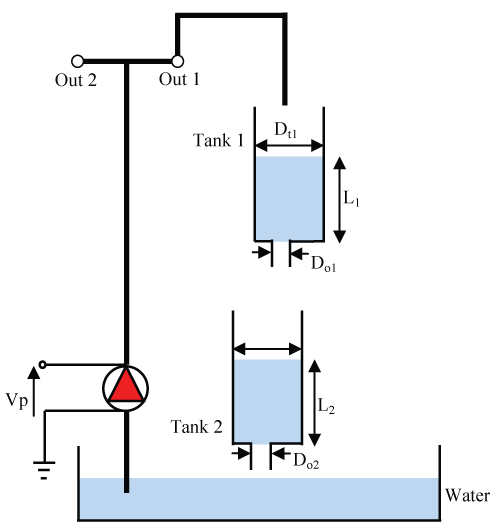
The Schematic for the CT system under study is shown in Figure 1. The two cylindrical tanks have uniform cross-sectional area and orifice diameter.

The CT system has an integrated pumping system and a reservoir (basin). The pumping system pumps water vertically through the piping system to tank 1. The two tanks are configured in such a way that tank 1 feeds tank 2 while tank 2 feeds the water reservoir at the base. The flow out of each tank is through the small orifice outlet located at the bottom of each tank. The liquid level in each tank is measured using pressure sensor mounted at the bottom of each tank. It is assumed that the pumping rate is directly proportional to the flow rate. The control objective in this context is to achieve optimum liquid level in tank 2 by manipulating the pump flow rate as manipulated variable. The list of constants and parameters that are associated with the CT system are given by Table 1.

System Dynamic Modelling

Nonlinear dynamic modelling

At this juncture, we present the dynamic modelling of the nonlinear CT system. The flow into tank 1 is given by Eq. 1 [15]

$f_{in1}\text{ = }{k}_p{v}_p\text{ (1)}$

By making use of Bernoulli’s equation, the flow velocity through the orifice of tank 1 and that of tank 2 are given by Eq. 2 and Eq. 3 respectively.

$v_o\text{ = }\sqrt{2g{l}_1}\text{ (2)}$

$v_o\text{ = }\sqrt{2g{l}_2}\text{ (3)}$

Using Eq. 2, the flow rate out of tank 1 is given by Eq. 4 as

$f_{o1}\text{ = }{A}_{o1}\sqrt{2g{l}_1}\text{ (4)}$

Similarly, using Eq. 3 the flow rate out of tank 2 is given by Eq. 5 as

$f_{o2}\text{ = }{A}_{o2}\sqrt{2gl2}\text{ (5)}$

Using mass balance equation where constant density is assumed, the rate of change in liquid level in tank 1 is given by

$\frac{d{l}_1}{dt}\text{ = }\frac{f_{in1}-f_{o1}}{A{t}_1}\text{ (6)}$

Substituting Eq. 1 and Eq. 4 into Eq. 6 yields

$\frac{d{l}_1}{dt}\text{ = }\frac{k_p{v}_p}{A{t}_1}-\frac{A_{o1}\sqrt{2g{l}_1}}{A{t}_1}\text{ (7)}$

Using mass balance equation where constant density is assumed, the rate of change in liquid level in tank 2 is given by

$\frac{d{l}_2}{dt}\text{ = }\frac{f_{in2}-f_{o2}}{A{t}_2}\text{ (8)}$

For the CT arrangement given by Figure 1, input flow to tank 2 is equal to output flow from tank 2, hence

$f_{in2}\text{ = }{f}_{o1}\text{ (9)}$

Substituting Eq. 5 and Eq. 9 into Eq. 8 gives

$$\frac{d{l}_2}{dt}\text{ = }\frac{A_{o1}\sqrt{2g{l}_1}}{A{t}_2}-\frac{A_{o2}\sqrt{2g{l}_2}}{A{t}_2}\text{ (10)}$$

Nonlinear Eq. 7 and Eq. 10 describe the dynamics of the CT system.

Dynamic model linearization

The linearization of the nonlinear CT system model was conducted based on Taylor series approximation given by Eq. 11

$$f\left(\gamma \right)\text{ = }f\left({\gamma }_0\right)+\left(\gamma -{\gamma }_0\right)f^{\prime }\left({\gamma }_0\right)+\dots +\frac{{\left(\gamma -{\gamma }_0\right)}^n}{n!}{f}^n\left({\gamma }_0\right)\text{ (11)}$$

From Eq. 7 and Eq. 10 we make the following substitutions for the purpose of simplicity:

$${\alpha }_1\text{ = }\frac{-A_{o1}}{A{t}_1}\sqrt{2g},{\alpha }_2\text{ = }\frac{-A_{o2}}{A{t}_2}\sqrt{2g}\text{ (12)}$$

$${\beta }_1\text{ = }\frac{k_p}{A{t}_1},{\beta }_2\text{ = }\frac{A_{o1}}{A{t}_2}\sqrt{2g}\text{ (13)}$$

Hence Eq. 7 and Eq. 10 can be presented as Eq. 14 and Eq. 15 respectively

$$\frac{d{l}_1}{dt}\text{ = }{\alpha }_1\sqrt{l_1}+{\beta }_1{v}_p\text{ (14)}$$

$$\frac{d{l}_2}{dt}\text{ = }{\alpha }_2\sqrt{l_2}+{\beta }_2\sqrt{l_1}\text{ (15)}$$

By using Taylor series approximation (given by Eq. 11), the nonlinear terms in Eq. 14 and 15 are given by

$$\sqrt{l_1}\approx \sqrt{l_{1ss}}+\frac{1}{2\sqrt{l_{1ss}}}\left(l_1-l_{1ss}\right)\text{ (16)}$$

$$\sqrt{l_2}\approx \sqrt{l_{2ss}}+\frac{1}{2\sqrt{l_{2ss}}}\left(l_2-l_{2ss}\right)\text{ (17)}$$

Substituting Eq. 16 and Eq. 17 into Eq. 14 and Eq. 15 yields

$$\frac{d{l}_1}{dt}\text{ = }{\alpha }_1\left(\sqrt{l_{1ss}}+\frac{1}{2\sqrt{l_{1ss}}}\left(l_1-l_{1ss}\right)\right)+{\beta }_1{v}_p\text{ (18)}$$

$$\frac{d{l}_2}{dt}\text{ = }{\alpha }_2\left(\sqrt{l_{2ss}}+\frac{1}{2\sqrt{l_{2ss}}}\left(l_2-l_{2ss}\right)\right)+{\beta }_2\sqrt{l_{1ss}}+\frac{{\beta }_2}{2\sqrt{l_{1ss}}}\left(l_1-l_{1ss}\right)\text{ (19)}$$

Where l_1ss and l_2ss denote the steady state operating points for the liquid levels in tank 1 and tank 2 respectively.

At steady state conditions, l₁ = l_1ss and l₂ = l_2ss, hence Eq. 18 and Eq. 19 become Eq. 20 and Eq. 21 respectively.

$$0\text{ = }{\alpha }_1\sqrt{l_{1ss}}+{\beta }_1{v}_{pss}\text{ (20)}$$

$$0\text{ = }{\alpha }_2\sqrt{l_{2ss}}+{\beta }_2\sqrt{l_{1ss}}\text{ (21)}$$

By subtracting Eq. 20 and Eq. 21 respectively from Eq. 18 and Eq. 19 and making the substitutions

$$l_1^{\text{'}}\text{ = }\left(l_1-l_{1ss}\right)$$ $$l_2^{\text{'}}\text{ = }\left(l_2-l_{2ss}\right)$$ and $$v_p^{\text{'}}\text{ = }\left(v_p-v_{pss}\right)$$ gives

$$\frac{d{l}_1^{\text{'}}}{dt}\text{ = }\frac{{\alpha }_1}{2\sqrt{l_{1ss}}}{l}_1^{\text{'}}+{\beta }_1{v}_p^{\text{'}}\text{ (22)}$$

$$\frac{d{l}_2^{\text{'}}}{dt}\text{ = }\frac{{\alpha }_2}{2\sqrt{l_{2ss}}}{l}_2^{\text{'}}+\frac{{\beta }_2}{2\sqrt{l_{1ss}}}{l}_1^{\text{'}}\text{ (23)}$$

By taking Laplace transform of Eq. 22 and Eq. 23, rearranging and substituting the values of the CT system parameters and constant given by Table 2, the transfer function for the CT system from pump to tank 2 is given by

$$G\left(s\right)\text{ = }\frac{6.9816\times {10}^{-3}}{s^2+0.1313s+4.3095\times {10}^{-3}}\text{ (24)}$$

Equation 24 represents the linear model for the CT system obtained analytically. Another method that can be used for obtaining a linear first order approximate model with deadtime for the nonlinear CT system is empirical method. The method is similar to system identification but it is more applicable in process control. Because most of the process in process control are associated with deadtime. To design a linear controller for a process linear model is required. In this study we used linear approximated model obtained using empirical method to designed linear controllers and nonlinear model which is the actual model to designed nonlinear controllers. Using this approach, the linear first order approximate model with deadtime model of the CT can be presented using, Eq. 25 obtained from [18] as

$$G\left(s\right)\text{ = }\frac{K_{dc}{e}^{-\theta s}}{\tau s+1}\text{ (25)}$$

Where K_dc, θ and τ are plant dc-gain, deadtime and plant time constant respectively. K_dc, θ and τ were obtained using Eq. 26, Eq. 27 and Eq. 28 respectively.

$$K_{dc}\text{ = }\frac{Changein{l}_2}{Changein{v}_p}\text{ = }\frac{\Delta l_2}{\Delta v_p}\text{ (26)}$$

$$\tau \text{ = 1}\text{.5}\left(t_{63\%}-t_{28\%}\right)\text{ (27)}$$

$$\theta \text{ = }{t}_{63\%}-\tau \text{ (28)}$$

Where t_63% and t_28% are times taken for the system’s output to reach 63% and 28% steady state value respectively.

By applying a step change input perturbation to the nonlinear model for the CT system, the parameters for the model given by Eq. 25 were calculated using Eq. 26 to Eq. 28 by extracting data from process reaction curve of the nonlinear model for the CT system. The empirical model for the CT is given by Eq. 29

$$G\left(s\right)\text{ = }\frac{1.62e^{-1.3s}}{24s+1}\text{ (29)}$$

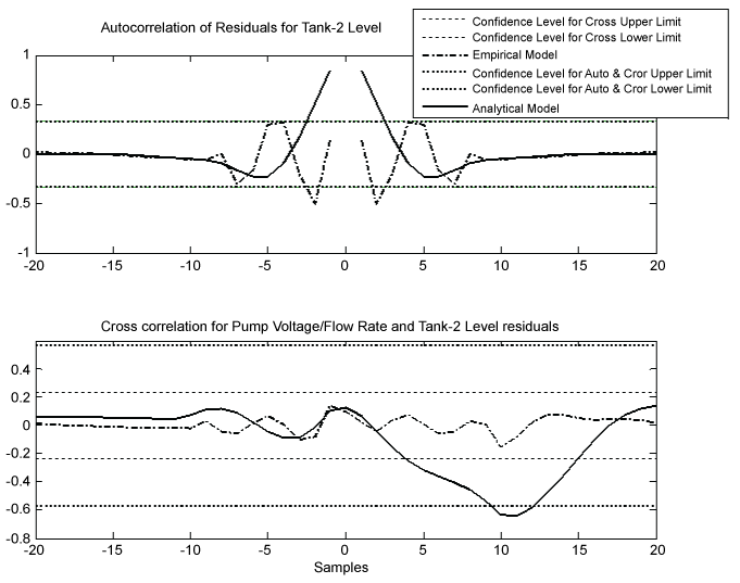
Residual analysis and Auto correlation analysis were employed as shown in Figure 2 to investigate the accuracy of the linear models for the CT system given by Eq. 24 and Eq. 29.

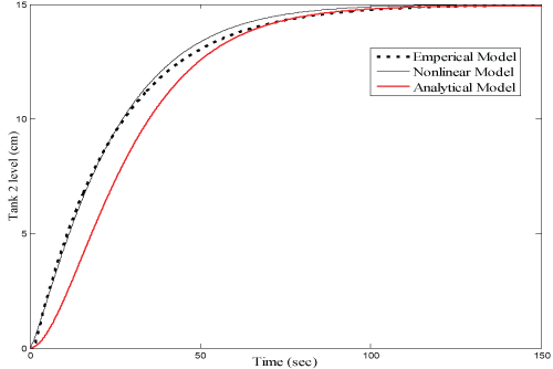
The models were compared with the nonlinear model for the CT system (Eq.7 and Eq.10) as shown in Figure 3 based on Final Prediction Error (FPE), Mean-Square Error (MSE), Integral Absolute Error (IAE), Mean Absolute Error (MAE) and Confidence Level (CFL). The comparisons for the results are given by Table 2.

Based on the model validation techniques employed, the empirical model was observed to deviate from the nonlinear model less when compared to the deviation of the analytical model and indeed Deadtime can be clear seen in the empirical model as most of the processes are associated with Deadtime naturally.

Control Systems Design

At this point we present the proposed control strategies. The main control objective is to maintain the liquid level in tank 2 at desired level by adjusting the pump flow rate. The control designs have been categorized into two; category one control systems and category two control systems. In category one, PI controllers based on PP, ZN and CC tuning rules have been proposed, while in category two advanced control systems based on PI + FF and MPC have been proposed. The requirements are that the control systems should satisfy the following specifications:

• The steady state error should be zero, hence e_ss = 0

• The operating point in tank 2 should be 15 cm, thus L₂ = 15 cm

• The percentage overshot in tank 2 to less than 10%, thus PO₂ ≤ 10%

• Settling time for tank 2 should be less than 20 seconds, thus; Ts 2 ≤ 20 sec

PI control system designs

The role played by PP control is it stabilizes an unstable system stable or improves its transient response performance by placing the system closed-loop poles to the left half of the s-plane [19].

The transfer function for a parallel form PI controller is given by [3]

$$G_c\left(s\right)\text{ = }{K}_c+\frac{K_I}{s}\text{ (30)}$$

The Deadtime for the linear model of Eq. 29 is very negligible compared to the dominant time scale of the system. Hence, we can neglect the Deadtime without loss of generality.

By using the PI controller given by Eq. 30 and the CT plant equation given by Eq. 29, the closed-loop characteristic equation for the system is given as

$$s^2+\frac{\left(1+K_{dc}{K}_c\right)s}{\tau }+\frac{K_{dc}{K}_I}{\tau }\text{ = 0 (31)}$$

By comparing Eq. 31 with Eq. 32, the tuning parameter K_c and K_I for the PI controller can be obtained by means of pole placement where the desired characteristic equation is

$$s^2+2\xi {\omega }_{n}s+{\omega }_n^2\text{ = 0 (32)}$$

The value for the damping coefficient, $\xi$ and natural frequency, ${\omega }_n$ can be calculated by making use of the following relationship given by $\xi \text{ = }\frac{\left|1n\left(\frac{P{O}_2}{100}\right)\right|}{\sqrt{{\pi }^2+1n{\left(\frac{P{O}_2}{100}\right)}^2}};{\omega }_n\text{ = }\frac{4}{\xi T_S}\text{ (33)}$

The parameters $\xi$ and ${\omega }_n$ were obtained as 0.5912 and 0.3383 respectively. Similarly, solving for K_c and K_I gives 5.3087 and 1.6955 respectively. Hence, the PI controller transfer function is given by

$$G_c\left(s\right)\text{ = 5}\text{.3087+}\frac{1.6955}{s}\text{ (34)}$$

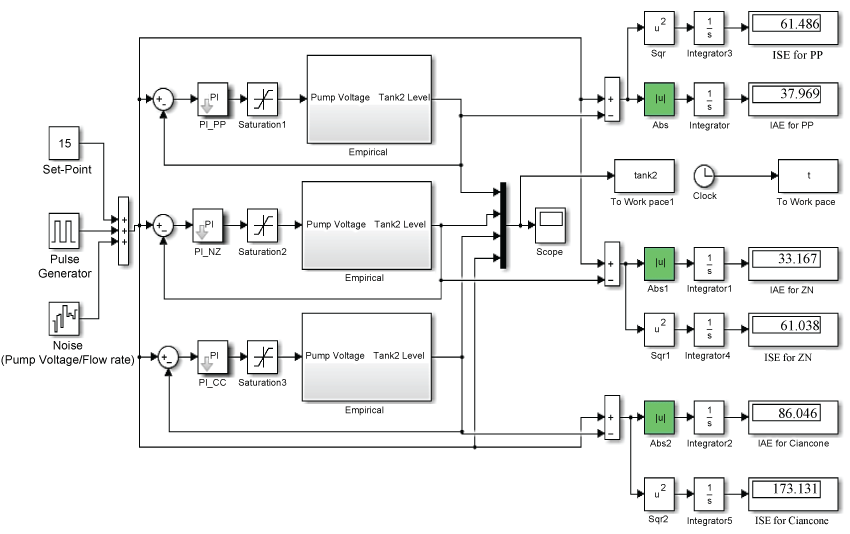
Similarly, ZN and CC tuning rule were implemented using Matlab/Simulink shown in Figure 4 for the purpose of investigating the tuning rule that will give the best response in terms of time response characteristics, minimal IAE and minimal ISE values.

The summary of the tuning parameters (K_c and K_I) for the PI controller based on the three tuning rules discussed is given by Table 3.

PI-plus-feedforward control systems design

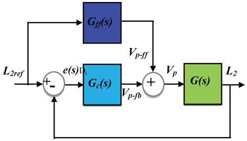
In this section, PI + FF control system design is presented. The structure of the PI + FF control strategy is given by Figure 5. FF control helps to compensate for the changes in load disturbance before they are detected by the Feedback (FB) control system. By doing this, the controlled variable (in this context, liquid level in tank 2) does not deviate considerably from its set point. Furthermore, the FF control is fully compatible with FB.

At steady-state conditions, the following modifications can be made to Eq. 10.

$$l_1\text{ = }{l}_{1ss}$$ $$l_2\text{ = }{l}_{2ss}$$ and $$i_2\text{ = 0 (35)}$$

Hence, Eq. 10 can be written as Eq. 36.

$$l_1\text{ = }{\left(\frac{A_{o2}}{A_{o1}}\right)}^2{l}_{1ss}\text{ (36)}$$

Equation 35 can be used to design FF controller for liquid level control in tank 2. The control problem requires us to compute the FF controller gain, k_ff2 using Eq. 36 as

$$k_{ff2}\text{ = }{\left(\frac{A_{o2}}{A_{o1}}\right)}^2\text{ (37)}$$

$$v_{pff2}\text{ = }{k}_{ff2}\sqrt{l_2}\text{ (38)}$$

Therefore, after incorporating FF controller to the CT system, the total input voltage to the system is the sum of the output voltage from the FF controller and that of FB controller.

MPC control system design based on GPC

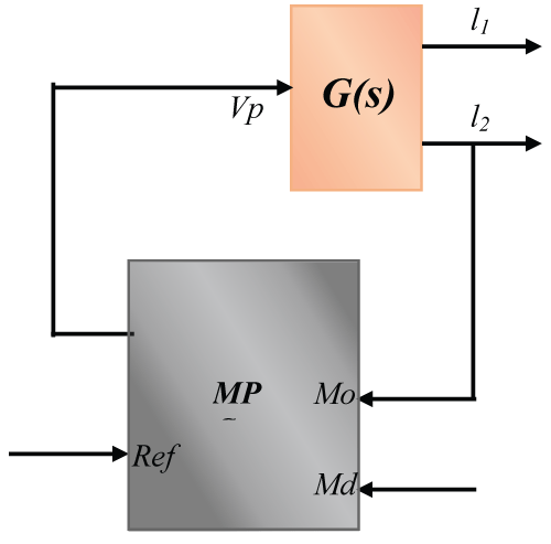
The structure of the MPC control strategy is given by Figure 6, where the measured variable (level in tank 2) is fed back and compared with the reference signal (level set-point).

In MPC control strategy the control problem is formulated based on Generalized Predictive Control (GPC). The discrete state-vector representation of the CT system can be expressed as

$$x_m\left(k+1\right)\text{ = }{A}_m{x}_m\left(k\right)+B_{m}u\left(k\right)\text{ (39)}$$

$$y_m\left(k\right)\text{ = }{C}_m{x}_m\left(k\right)\text{ (40)}$$

Where,

$$x_m\left(k\right)\text{ = }\left[\begin{array}{cc}{l}_1& \left(k\right)\\ l_2& \left(k\right)\end{array}\right]$$ $$y_m\left(k\right)\text{ = }\left[\begin{array}{cc}{l}_1& \left(k\right)\\ l_2& \left(k\right)\end{array}\right]$$ and $$u\left(k\right)\text{ = }{v}_p\left(k\right)\text{ (41)}$$

To design a predictive controller, u(k) needs to be adjusted. Hence Eq. 39 and Eq. 40 are augmented with an integrator as

$$\left[\begin{array}{cc}\Delta x_m& \left(k+1\right)\\ y_m& \left(k+1\right)\end{array}\right]\text{ = }\stackrel{A}{\overbrace{\left[\begin{array}{cc}{A}_m& 0_m^T\\ C_m{A}_m& 1\end{array}\right]}}\stackrel{x\left(k\right)}{\overbrace{\left[\begin{array}{cc}\Delta x_m& \left(k\right)\\ y_m& \left(k\right)\end{array}\right]}}+\stackrel{B}{\overbrace{\left[\begin{array}{c}{B}_m\\ C_m{B}_m\end{array}\right]}}\Delta u\left(k\right)\text{ (42)}$$

$$y_m\left(k\right)\text{ = }\stackrel{C}{\overbrace{\left[\begin{array}{cc}{0}_m& 1\end{array}\right]}}\left[\begin{array}{cc}\Delta x_m& \left(k\right)\\ y_m& \left(k\right)\end{array}\right]\text{ (43)}$$

Where,

$$0_m\text{ = }\left[0---0\right]$$

$$\Delta x_m\left(k+1\right)\text{ = }{x}_m\left(k+1\right)-x_m\left(k\right)$$

and if We connect x_m(k) to the output, then we can form a new state variable vector given as

$$x\left(k\right)\text{ = }{\left[\begin{array}{cc}\Delta x_m{\left(k\right)}^T& y_m\left(k\right)\end{array}\right]}^T$$

Where Δx_m refers to the difference of the state variable and is given by

$$\Delta x_m\left(k\right)\text{ = }{x}_m\left(k\right)-x_m\left(k-1\right)$$

Assuming current sampling instance Ki > 0, then the future states of the system can be computed using the equation given as

$$x\left(k_i+N_p|k_i\right)\text{ = }{A}^{N_P}x\left(k_i\right)+A^{N_P-1}B\Delta u\left(k_i\right)+A^{N_P-N_c}B\Delta u\left(k_i+N_c-1\right)\text{ (44)}$$

Where N_c refers to control horizon, N_p is the length of the optimized prediction window and Δu(k) is the difference of the control variables and is given by

$$\Delta u\left(k\right)=u\left(k\right)-u\left(k-1\right)$$

From Eq. 44 the output prediction can be expressed as

$$Y=Fx\left(k_i\right)+\Phi △U\text{ (45)}$$

where, $$Y={\left[\begin{array}{cccc}y\left(k_i+1|k_i\right)& y\left(k_i+2|k_i\right)& \mathrm{...}& y\left(k_i+N_p|k_i\right)\end{array}\right]}^T$$

$$\Delta U={\left[\begin{array}{cccc}\Delta u\left(k_i\right)& \Delta u\left(k_i+1\right)& \mathrm{...}& \Delta u\left(k_i+N_c-1\right)\end{array}\right]}^T$$

$$F=\left[\begin{array}{c}CA\\ C{A}^2\\ ⋮\\ C{A}^{N_p}\end{array}\right]$$ and $$\Phi =\left[\begin{array}{cccc}CB& 0& \cdots & 0\\ CAB& CB& \cdots & 0\\ ⋮& ⋮& \cdots & 0\\ C{A}^{N_p-1}B& C{A}^{N_p-2}B& \cdots & C{A}^{N_p-N_c}B\end{array}\right]$$

If we assume the data vector that contains the set-point information is given by Eq. 46 then the cost function reflecting the control objective function can be written as Eq. 47.

$$R_s{}^T=\underset{N_p}{\underbrace{\left[\begin{array}{cccc}1& 1& \cdots & 1\end{array}\right]}}r\left(k_i\right)\text{ (46)}$$

$$J={\left(R_s-Y\right)}^T\left(R_s-Y\right)+\Delta U^T{R}_d\Delta U\text{ (47)}$$

Where, $$R_d=r_w\times I_{N_c\times N_c}{,}_{}{r}_w\ge 0$$ R_d is used as a tuning parameter to achieve the desired closed-loop response.

The requirement is to find the change in control input, ΔU that will minimize the cost function, J using Eq. 47.

A rule of thumb for selecting an appropriate value for MPC controller prediction horizon, N_P is to select a value that is at least equal to the model settling time. For this reason, a value of 30 is a reasonable selection. The controller sampling period was selected as 0.1 seconds (corresponding to 10 Hz sampling frequency). Other MPC controller design parameters values are given by Table 4.

Results and Discussions

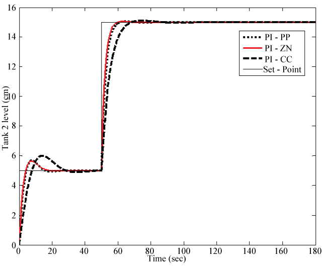
At this point, the results obtained in this work are presented. The accuracy of the two linear models (analytical and empirical) given by Eq. 24 and Eq. 29 derived from the nonlinear model given by Eq. 7 and Eq. 10 were investigated as shown previously in Figure 2 and Figure 3. Based on Figure 3, it can be seen that the empirical model is more accurate when compared to the analytical model. This can be attributed to the linearization approximations of the two nonlinear terms in Eq. 7 and Eq. 10, and also as a result of the fact that the analytical model does not account for the system time delay. To further support this argument, FPE, MSE, IAE, MAE and CFL values for modelling errors have been investigated and are given by Table 2 (above). The error values also showed that the empirical model was more accurate. Figure 7 shows the tracking control responses for PI controllers based on ZN, CC and PP tuning rules. Table 5 and Table 6 show the corresponding time response characteristics and IAE and ISE values respectively for the three PI tuning rules. Based on the results, it can be seen that ZN tuning rule have the lowest IAE and ISE value of 33.17 and 61.04 (Table 6). Settling time for ZN, CC and PP rules were 17 seconds, 37 seconds and 15 seconds respectively, Overshoots of 8%, 26% and 14% were observed for ZN, CC and PP respectively. However steady state errors were notice in both the cases. Furthermore, it can be noticed that all the PI tuning rules did not give us a PI controller that satisfies our 20 seconds settling time and 10% overshoot.

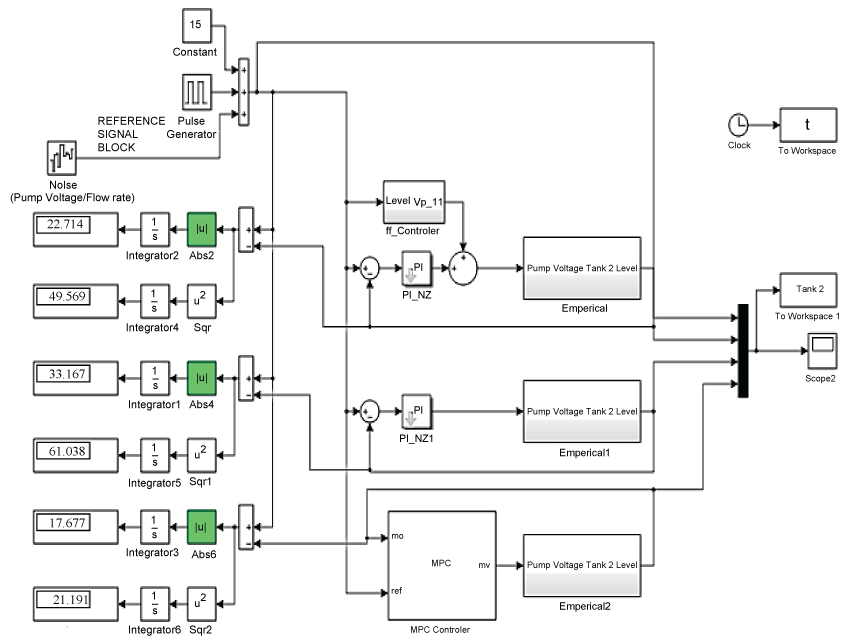
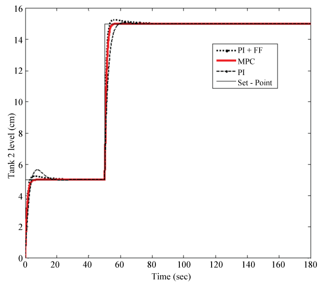
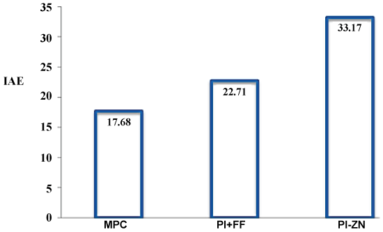
It was assumed that overshoot needs more attention, hence ZN tuning was considered “better”. For this reason, an improved PI controller (by means of FF controller incorporation) and MPC controller were investigated for faster and a more robust performance using Matlab/Simulink block diagram shown in Figure 8. Figure 9 shows the tracking control responses for ZN based PI, PI + FF and MPC controllers. Based on the results presented in Figure 9 and Table 7, an improvement was observed after FF controller was added to the PI feedback controller. However, MPC response was more superior compared the responses for PI and PI + FF controllers. In point of fact, based on ISE and IAE values for PI, PI + FF and MPC control strategies given by Table 7 and Figure 10, it can be seen that MPC has the smallest ISE (21.19) and IAE (17.68) values, hence it shows that MPC response was better.

Conclusion

From the nonlinear dynamic model, the transfer function models for the Coupled-Tank system based on analytical and empirical methods have been established. FPE, MSE, IAE, MAE and CFL were employed for the purpose of investigating the accuracy of the empirical and analytical models. Hence, based on FPE, MSE, IAE, MAE and CFL error levels presented in Table 2 above, it can be concluded that the empirical model was more accurate in this context. PI controllers for liquid level control in tank 2 based on three tuning methods (ZN, CC and PP) have been designed using MATLAB/Simulink. In this context, PI based on ZN tuning method’s response was more acceptable as it has been investigated based on IAE values, ISE values and time response characteristics.

The PI controller was unable to satisfy all the control objectives. To further improve the robustness of the PI - ZN, a FF controller was incorporated to the PI controller. The response for the PI + FF controller was compared to the response obtained by MPC for level control in tank 2. Based on ISE values, IAE values and time response charateristics, the performances of the ZN - PI, PI + FF and MPC controllers were investigated. It was observed that, the PI + FF controller and MPC controller can be used to achieve all the control objectives. However, the response by MPC controller was more acceptable in terms of time response characteristics where 0% overshot and 4 seconds settling time were recorded. ISE and IAE values also confirmed the MPC controller was more rubost.

Author Contributions

All authors contributed equally in the presented research work.

Conflicts of Interest

The authors declare no conflict of interest.

References

1. Liang L (2011) The application of fuzzy PID controller in coupled-tank liquid-level control system. 2011 International Conference on Electronics, Communications and Control (ICECC) 2894-2897.
2. Ramli MS, Ahmad MA, Ismail TR (2009) Comparison of swarm adaptive neural network control of a coupled tank liquid level system. 2009 International Conference on Computer Technology and Development (ICCTD) 130-135.
3. Abiodun FT, Habeeb BS, Mikail OO, et al. (2013) Control of a Two Layered Coupled Tank : Application of IMC, IMC-PI and Pole-Placement PI Controllers. Int J Multidiscip Sci Eng 4: 1-6.
4. Jalil MHA, Marzaki MH, Kasuan N, et al. (2013) Implementation of Aanti Windup Sscheme on PID Controller for Regulating Temperature of Glycerin Bleaching Process. 2013 IEEE 3rd International Conference on System Engineering and Technology (ICSET) 113-117.
5. Katal N, Kumar P, Narayan S (2014) Optimal PID Controller for Coupled-Tank Liquid- Level Control System using Bat Algorithm. 2014 International Conference on Power, Control and Embedded Systems (ICPCES) 1-4.
6. Wahyudi MS, Fadhil M (2007) Robust Anti-windup PID Control of a Couple Industrial Tank System. 2007 International Conference on Mechanical Engineering (ICME2007) 1-4.
7. Mahyuddin MN, Arshad MR, Mohamed Z (2007) Simulation of Direct Model Reference Adaptive Control on a Coupled-Tank System using Nonlinear Plant Model. International Conference on Control, Instrumentation and Mechatronics Engineering (CIM’07) 569-576.
8. Selamat NA, Daud FS, Jaafar HI, et al. (2015) Comparison of LQR and PID Controller Tuning Using PSO for Coupled Tank System. 2015 IEEE 11th International Colloquium on Signal Processing & its Applications (CSPA) 6-8.
9. Alhassan A, Danapalasingam KA, Shehu M, et al. (2015) Comparing the Performance of Sway Control Using ZV Input Shaper and LQR on Gantry Cranes. 9th Asia Modelling Symposium 61-66.
10. Shehu M, Ahmad MR, Shehu A, et al. (2015) LQR , Double-PID and Pole Placement Stabilization and Tracking Control of Single Link Inverted Pendulum. 2015 IEEE International Conference on Control System, Computing and Engineering (ICCSCE) 27-29.
11. Gupta H, Verma OP (2012) Intelligent Controller for Coupled Tank System. Int J Adv Res Comput Sci Softw Eng 2: 154-157.
12. Arif MU, Iqbal DK, Kadri MB (2014) Adaptive Online Fuzzy Controller for a Coupled Tank System. 2014 IEEE 17th International Multi-Topic Conference (INMIC) 338-343.
13. Abbas H, Asghar S, Qamar S (2012) Sliding Mode Control for Coupled-Tank Liquid Level Control System. 2012 10th International Conference on Frontiers of Information Technology (FIT) 325-330.
14. Musmade B, Patre B (2013) Feedforward-plus-Sliding Mode Controller Design with Experimental Application of Coupled Tank System. Trans Inst Meas Control 35: 1058-1067.
15. Salunkhe SM, Kurode SR, Bhole VB (2015) Robust control of liquid level in coupled tank system using smooth first order sliding modes. 2015 International Conference on Industrial Instrumentation and Control (ICIC) 1647-1650.
16. Essahafi M (2014) Model Predictive Control (MPC) Applied To Coupled Tank Liquid Level System. Procedia Technology 22: 614-622.
17. John JA, Jaffar NE, Francis RM (2015) Modelling and Control of Coupled Tank Liquid Level System using Backstepping Method. Int J Eng Res Technol 4: 667-671.
18. Juneja PK, Ray AK, Mitra R (2010) Deadtime Modeling for First Order Plus Dead Time Process in a Process Industry. Int J Comp Sci & Comm 1: 167-169.
19. Ogata K (2015) Modern Control Engineering. (5th edn), Prentice Hall, New Jersy.