Occupational and Residential Exposures to Infrasound and Low Frequency Noise in Aerospace Professionals: Flawed Assumptions, Inappropriate Quantification of Acoustic Environments, and the Inability to Determine Dose-Response Values

Abstract

Professionals within the aerospace industry are often required to remain within acoustic environments characterized by a predominance of low frequency and infrasound components. Safety-and-health-in-the-workplace officials are mindful of the threat these extreme environments can pose to the hearing function. Noise-exposed professionals are, therefore, frequently provided with a plethora of ear protection devices to shield this vital human sense. The vast majority of noise-protection guidelines and regulations, however, are inappropriate to protect aerospace professionals against acoustic environments rich in Infrasound and Low Frequency Noise (ILFN) because they are based on the flawed premises that ILFN only affects humans through the aural pathway, and that dynamics are unimportant. Consequently, the numerical values needed to estimate potential harm to people (dose-response levels) are not routinely obtained or assessed. The goals of this paper are to inform a) Aerospace professionals who are consistently exposed to acoustic environments rich in ILFN, about how this agent of disease is being incorrectly evaluated leading to improper worker protection; and b) Noise control and health professionals who work within the aerospace industry, about new methodologies in acoustical evaluations pertinent to infrasound and low frequency noise dose-response values. New sources of ILFN are increasingly present in the vicinity of residential environments, quite possibly eliminating biological recovery periods for noise-exposed aerospace workers. This paper details the inadequacy of the use of the dBA metric and 1/3-octave-band analysis when protecting workers (and the public) against excessive ILFN exposures. The complexities associated with acoustical evaluation in conjunction with objective and pertinent medical outcomes are discussed, and the need for narrowband analyses in routine evaluation procedures is emphasized.

Keywords

Infrasound, Low frequency noise, dBA, Narrow-band analysis, Occupational exposure, Environmental exposure, Pathology

Introduction

In a widely read paper published by the World Health Organization (WHO), Burden of disease from environmental noise [1], the long-term effects of excessive noise exposure were shown to be worrisome, at best. Historically, noise exposures were deemed to be detrimental to the hearing function, i.e., people exposed to loud noise were more likely to become deaf, or hearing impaired. Consequently, only a portion of the acoustical spectrum was focused upon - the one containing the frequencies responsible for hearing loss.

This restricted segment of the acoustical spectrum, called ‘the audible portion’, ranges from 20 Hz to 20 kHz. Within this wide range of frequencies, though, not all of them are equally responsible for deafness or hearing loss. Deafness due to excessive noise exposure is predominantly a consequence of loss of hearing function within the 250-8000 Hz range, i.e., deafness at frequencies above 8000 Hz or below 250 Hz is not as relevant for speech intelligibility as are those contained within the 250-8000 Hz range. Health-related acoustical evaluations were thus urged to focus on this particular range of frequencies. This required measuring instrumentation that would eliminate all the frequencies considered irrelevant to human hearing impairment, i.e., all extending beyond the 250-8000 Hz range. Infrasound and Low Frequency Noise (ILFN) (< 200 Hz) was, therefore, deemed irrelevant for the purposes of protecting human health.

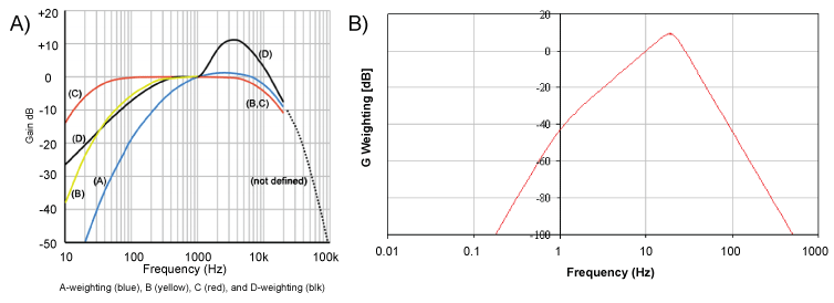
The human ear responds to sound non-linearly, both in terms of frequency and sound pressure level. Hence the development of filters (with specific frequency-weighting curves) designed to simulate the non-linear sensitivity of human hearing. Measuring sound levels with one of these filters would then better represent the human perception of the sound. Figure 1 shows examples of A-, B-, C- and D-weighting curves (Figure 1A), and the more recent G-weighting curve, developed for ILFN-rich environments (Figure 1B).

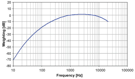
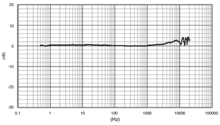
Under the dBA metric, acoustical energy contained in other portions of the spectrum are de-emphasized (< 250 Hz and > 8000 Hz) or deemed irrelevant for evaluation (< 20 Hz, or ‘infrasound’, and > 20 kHz, or ‘ultrasound’). Regulations have been guided by these principles, leading to the ubiquitous capture of information within the restricted segment of the acoustical spectrum (20 Hz - 20 kHz), and with the A-weighting being applied. Figure 2 shows the frequency response curve for the A-weighting filter, which is relatively flat between 800 - 8000 Hz. When measuring frequencies < 200 Hz with an incorporated A-weighting network, the numerical value obtained for the sound pressure level presents with a 10 to 70 dB error. While the A-weighting system seems to yield good results for hearing protection, it is clearly inadequate for assessing the amount of acoustical energy present in the ILFN ranges, because these lower frequency components are discounted; for example, a reduction of about 70 dB at 10 Hz (Figure 2).

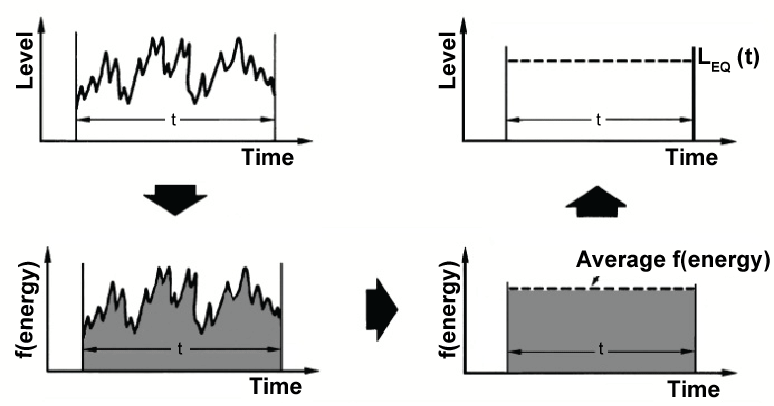
Two additional difficulties exist when evaluating acoustic environments: a) They are constantly varying in time (seconds); and b) They do so continuously across the entire acoustical spectrum. Hence, to enable analyses, both time and frequency parameters need to be segmented. To transform a time-varying signal into some manageable number, the concept of time-averaged sound level was developed (Leq). Figure 3 sketches the mathematical treatment given to a time-varying signal, such as an airborne pressure wave.

Occupational and health issues consider long term exposures in LAeq (A-weighted, time-averaged sound level), and allow short testing samples as representative of an 8-hour day exposure. Many environmental regulations, on the other hand, mandate 10-minute time averages of LAeq, so that values are not skewed by intermittent loud sounds. Either way, information on the dynamic, time-dependent portion of the acoustic environment is diluted when the signal has significant variations in time and is segmented into 10 min or 1 hour windows.

The ‘audible’ frequency spectrum was segmented into ‘octave’ and ‘1/3-octave’ bands, facilitating further analyses for noise control evaluations. Although data resolution was improved with the 1/3-octave bands analyses, this methodology still only provides a crude resolution of the acoustic environment. Figure 4A compares octave band and 1/3-octave band measurements. In the pre-digital era, investigations of finer resolution were very involved, complex and beyond the means of general acoustic investigations.

When no weighting network is incorporated into the acoustic signal capture, measurements are un-weighted (unfiltered), and the metric written as dBLin (linear) to distinguish it from other forms of deciBel. Figure 4B shows the difference between the overall dBA and dBLin levels in an environment where ILFN components are predominant. While the overall dBA level reflects what a human would hear, the dBLin level reflects the acoustical energy to which the body is exposed.

There are further limitations related to accuracy when the frequency spectrum is segmented into 1/3-octaves. This method ignores the exact problem that impulsive sounds (perceived as irritating or not) will be invisible in such LAeq measures. For example, a single gun-shot would have little, if any, impact upon a 10 minute dBA-level average but would hardly fail to wake a sleeper. In terms of urban population health, the inappropriateness of using the dBA metric to assess ILFN-rich environments was recognized almost two decades ago by the WHO: “When prominent low-frequency components are present, measures based on A-weighting are inappropriate. However, the difference between dBC (or dBLin) and dBA will give crude information about the presence of low-frequency components in noise” [2].

It is not uncommon to address the maximum dBC level or dBLin level in order to ‘squeeze out’ more acoustical information from measurements obtained with legislated methodologies. However, a more detailed numerical characterization of acoustic environments within the ILFN range is needed, in order to establish dose-response values for human protection.

Interface between acoustical phenomena and the human body

The WHO publication International Classification of Diseases (ICD-10 2016) [3], dedicates Chapter 20 to “External causes of morbidity and mortality”, and block W20-W49 refers to “Exposure to inanimate mechanical forces”:

W42 - Exposure to noise Incl.: Sound waves, Supersonic waves

W43 - Exposure to vibration Incl.: Infrasound waves [3].

Airborne acoustical phenomena interact with the human body when mechanical coupling occurs between the oncoming mechanical force and a particular tissue or tissue system of the human body. This brings the issue of ILFN health effects into the field of materials engineering. Biological tissues are viscoelastic materials, i.e., they possess the properties of creep, relaxation and hysteresisa. Moreover, they feature anisotropy, i.e., equal forces applied in different directions yield different results. Biological material, particularly when considering whole-body effects, cannot be modeled as a simple Hookean elastic^a; and neither can its response when immersed in an ILFN-rich environment.

Prof. Donald Ingber (Wyss Institute, Harvard University), proposed decades ago that animal cells were constructed in accordance with principles of tensegrity [4-6], i.e., architectures consisting of elements providing continuous tension, and elements providing discontinuous compression [7]. By modeling the cell as a tensegrity structure instead of the prior, elastic continuum model, it was possible to begin to understand cellular mechanotransduction, i.e., inter- and intra-cellular communication established via mechanical signals, as opposed to biochemical signals [8,9, for example]. Mechanotransduction and cellular tensegrity architectures are essential to understanding the specific structural changes in ILFN-exposed cells, as seen through light and electron microscopy [10-12]. These mechanically-induced cellular effects are not accounted for under current noise protection legislation, guidelines and procedures, as they do not respond to acoustical energy via the aural-perception pathway.

Mechanical coupling between airborne pressure waves and the human body is known to occur at the ear; the design of which is an engineering marvel. Mechanical coupling between airborne pressure waves and other regions of the body are acknowledged to exist only if the acoustic energy is at sufficient amplitude (i.e., if the event is perceivable by human senses), otherwise, effects are (perhaps erroneously) considered to be irrelevant or non-existent.

The response of biological tissue to ILFN is frequency-dependent. An early example is a study conducted in 1969 (within the scope of the Soviet and US space programs), where dogs were exposed to ILFN-rich environments at sound pressure levels ranging from 105 to 155 dB. This induced multiple hemorrhages in the lung tissue that “never exceeded 3 mm in diameter” [13]. Increasing the dB-level of the environment did not increase the size of the hemorrhagic areas, but rather, their number. In the early 1990’s, Professors Nekhoroshev and Glinchikov (St. Petersburg Academy of Sciences, Russia) exposed laboratory animals to infrasound (8-16 Hz) at 120-140 dB, for 3 hr daily, for 1, 5, 10, 15, 25, and 40 days, and found different morphofunctional changes in the cellular structures of myocardium and liver tissues when compared to controls [14,15]. These changes varied with frequency, exposure time and exposure level. For the past three decades, another team led by pathologist Col. Castelo Branco (Portuguese Air Force), has systematically studied both workers and animal models exposed to ILFN. As a result, the clinical evolution of the signs and symptoms consistently observed in aeronautical technicians was established in 1999 [16], supported by numerous collateral studies in human populations and animal models in subsequent years [17-19]. Since then, this ILFN-induced pathology, (termed Vibroacoustic Disease - VAD), has also been identified (as per objective clinical testing) in residential settings [20-22].

Certain, narrow frequency ranges can elicit a specific response from one type of tissue and not another, located adjacently, because each type of material has its own creep, relaxation and hysteresis coefficients^a. Each tissue type also possesses its own mechanical resonance frequency. Hence, at the electron microscopy level of ILFN-exposed tissue, the re-organization of inter- and intra-cellular architectures seem to reflect a mechanical reinforcement required to maintain structural integrity [23,24].

In Workplace Safety, vibration is considered as that which is transmitted into the human body through solid-to-solid contact, i.e., contact with a chain-saw (hand-arm vibration) or a vibrating platform (whole-body vibration). To measure vibration, accelerometers are used instead of microphones. With ILFN, impacts to the human body occur via a different interface: air-to-solid, or rather, air-to-composite viscoelastic material. Modeling human response to ILFN exposure based on solid-to-solid interfaces has not, therefore, proven very successful.

ILFN dose-response values - the need for narrow-band analyses

Dose-responses for ILFN exposures must be frequency dependent if they are to properly protect humans from excessive exposure to ILFN-rich environments. The determination of dose-responses for ILFN exposure has been scientifically impossible to achieve, however, because the ILFN in itself is not being quantified during routine acoustical evaluations. This is the point where the ILFN-rich occupational and environmental exposures meet. Both require precise ILFN measurements if human populations are to be properly protected from this agent of disease, whether at work or in the home.

For decades, the biomedical world has been in dire need for proper scientific instrumentation to objectively quantify ILFN-rich acoustic environments. Given that current instrumentation discards much of the information that characterizes an acoustic environment (at the behest of regulations) precluding any real scientific analysis, it becomes obvious that current general-sound-level measurement instrumentation is not suited to requirements.

The limitations of dBA methodology and 1/3-octave segmentation with respect to ILFN, can be resolved by the application of analyses using no weighting and by a proper signal capturing of the acoustic environment. This would allow a more precise identification of events that occur within frequency bands that are narrower than the 1/3-octave segmentation, and of periodic signals that occur in the time domain. Narrow band analyses can provide information that would permit the identification of discrete signals (e.g., tones or harmonics) forming acoustic signatures that are not evident with the dBA-1/3-octave methodology [25,26]. This is shown in the next sections.

Material and Methods

Instrumentation

The equipment used for acoustic capture was a SAM Scribe Full Spectrum (FS) system (Model: Mk1, Atkinson & Rapley, Palmerston North, New Zealand) [27,28]. It consists of a two-channel device that can measure at sampling rates up to 44.1 kHz, and that delivers data streams via USB to a Windows notebook computer, storing it as uncompressed wav files to hard disk. GPS information is also stored as metadata in the files, and this includes a digital signature. The system can accurately record from 0.1-1000 Hz, as per the manufacturer frequency response of the two electrets condenser microphones (custom-made Model No.: EM246ASS’Y, Primo Co, Ltd, Tokyo, Japan), Figure 5 [29].

The SAM Scribe FS unit has two switches: one enables a 1 Hz high-pass filter to remove unwanted ‘micro-barom’ events^b below 1 Hz, and the other enables a + 20 dB gain boost. All measurements were conducted with the 1 Hz filter enabled and with the 20 dB gain boost disabled. All measurements are reported from 1-800 Hz, and were captured with a sampling rate of 11.025 kHz.

Measurement methodology

All measurements were recorded to uncompressed wav file including the required reference calibration tone prior to and after measurements. Calibration tones were produced with a Type I calibrator (part of the SAM Scribe system) at 1000 Hz/94 dB. Calibration of the system rests on the manufacturer’s frequency-response curve for the Primo microphone capsule (Figure 5) as well as comparison calibrations between 6.3 Hz and 1000 Hz of the full system against a Larsen-Davis 831 sound level meter with a current National Association of Testing Authorities (Australia) calibration certificate. The manufacturer’s frequency response curve shows that the microphone capsule is very close to linear over the 1-1000 Hz range used in this study.

Wind-shields were always placed on both microphones during measurements. Microphones were attached to tripods at approximately 1.5 m above the ground. After microphone positioning and initial calibration, at least three 10 min segments of data were captured at each location. Both microphones were placed at the same location, along the same axis, approximately 20 m apart from each other, as limited by cable distance (5 m + 15 m). One microphone (red) was always placed at approximately 22 m from the shed entrance, and the second microphone (blue) was placed at approximately 42 m from the shed entrance (see below).

Measurements were performed on a rotating basis between locations, and on different days - 16, 30, and 31 December, 2016. This acoustical evaluation is part of an international, citizen-based research effort into the health effects caused by excessive exposure to ILFN, and to which the authors contribute [30]. Within this context field-sites, such as this one, become available due to the efforts of citizen scientists.

Selection of locations

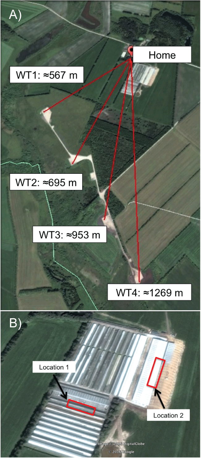
Data was gathered at a farm where the residential home is in the vicinity of the animal sheds (Figure 6). This preliminary data was selected for presentation due to: a) Its pedagogical strength for clarifying the difference between the type of data obtained through narrow-band analyses and legislated methodologies; b) The relative location of the home within the ILFN-rich acoustic environment (Figure 6A); and c) The possibility of gathering clues that may contribute to an explanation of different animal behavior in the presence of anthropogenic ILFN, depending on animal-shed location (Figure 6B).

The anthropogenic sources of ILFN in question are four, 3-MW Industrial Wind Turbines (IWT), 150 m in total height (hub height + ½ blade diameter) [31]. Figure 6A shows the relative positions of the home and animal sheds to the IWTs.

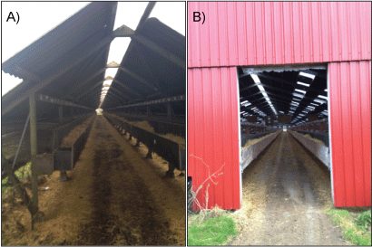
Locations 1 and 2 were suggested by the property owner as two locations where animal pups responded differently when IWT were rotating. Figure 7 shows the different construction types of the animal sheds in Location 1 and Location 2. Location 1 is a shed of older, wooden construction, with an interior space approximately 2.5 m in height and 75 m in length (Figure 7A). Location 2 is a more modern shed, mostly made of metal, with an interior space approximately 7.0 m in height, and 110 m in length (Figure 7B). Both contain water-supply systems for the animals that may produce specific and identifiable signatures within the acoustic environment. Since IWT rotation began, the property-owner has opted to maintain his breeding male animals in Location 1 rather than in Location 2. Table 1 tallies the measurements conducted at Location 1 and Location 2 in 2016.

Wind speed

In the case of this anthropogenic ILFN source (IWT), acoustical emissions output depend on the wind speed. (IWT power output graphs concurrent with these measurement sessions are unavailable).

Weather data was obtained from the Danish Meteorological Institute, corresponding to the monitoring tower closest to the farm, approximately 35 km away. Air pressure values were unavailable. Although the lack of in loco weather monitoring equipment led to imprecise numerical values, the goal of this data is not to relate specific wind speeds to specific IWT acoustical emissions, but rather to compare ILFN components under two different IWT regimens, at two different locations. Weather data is given in Table 2.

Results

Acoustic data was processed in Matlab (The MathWorks, USA) using narrow-band filters complying with the ANSI^® S1.11-2004 and IEC 61260:1995 standards, as well as FFTs.

Table 3 shows the measurement segments selected for scrutiny.

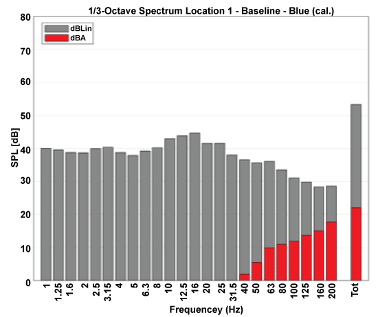
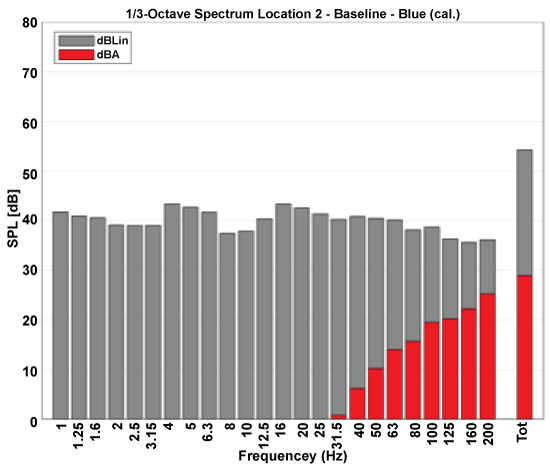
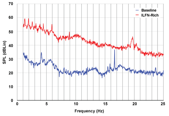
Figure 8 and Figure 9 show the traditional 1/3-octave spectra and the total dBA and dBLin levels, in Locations 1 and 2 respectively, under baseline conditions. Figure 10 and Figure 11 show the same numerical data but represented as narrow-band analyses.

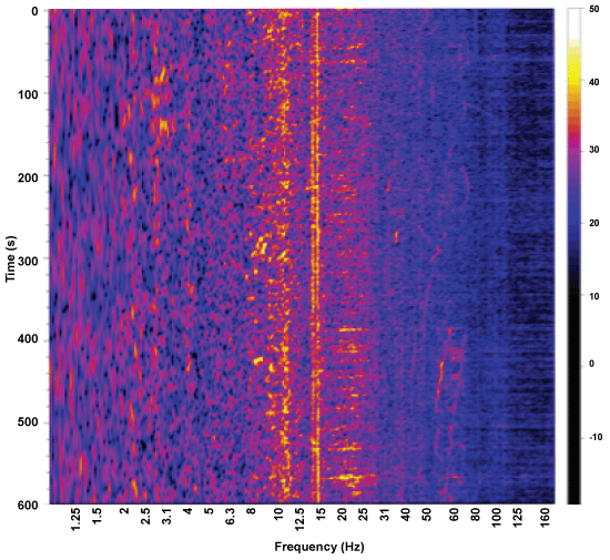
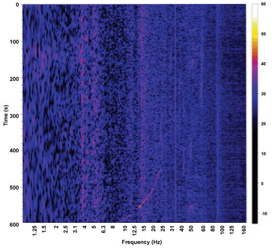
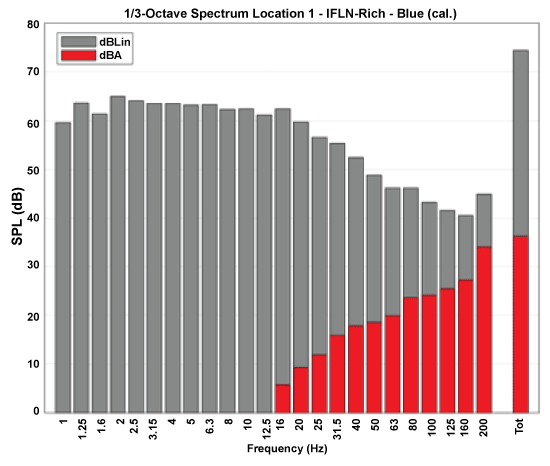
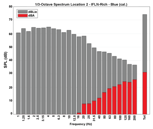
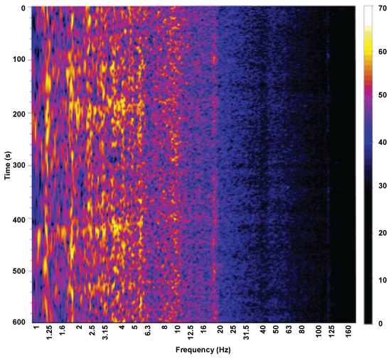
Similarly, Figure 12 and Figure 13 show the traditional 1/3-octave spectra and the total dBA and dBLin levels, in Locations 1 and 2 respectively, under ILFN-rich conditions. Figure 14 and Figure 15 show the same numerical data but represented as narrow-band analyses.

For ease of presentation herein, only the results corresponding to the blue microphone (placed at approximately 42 m from the entrance of the sheds) are presented.

Preliminary analysis

16 - 20 Hz:

Baseline:

Both Location 1 and Location 2 exhibit a continuous acoustical phenomenon with strong tonal characteristics occurring at around 16 Hz (Figure 10 and Figure 11). This could be associated with the water systems installed in the shed to feed the animals. Water could distinctly be heard running in the background in Location 1, but less so in Location 2.

ILFN-rich:

In Location 1, the continuous acoustical phenomenon, seen at around 16 Hz in the baseline (Figure 10), is still visible in Figure 14, but is no longer distinguishable from other acoustical events in Figure 15 (baseline, Figure 11). The apparent constancy of this acoustical feature in at least three of the four situations seems to suggest some permanent equipment, and hence the animal water supply system is a good contender.

Concurrent with the existence of IWT rotation, a new acoustical phenomenon, not present in either baseline, appears at 20 Hz and in both locations. The non-continuous coloring of this line shows that pressure level was not continuous. Further analysis (Figure 16 and Figure 17) shows that this 20 Hz phenomenon was equally prominent in Location 2 (newer shed) as in Location 1 (older shed).

10-12.5 Hz:

Baseline:

Given the continuous nature of the acoustical event that occurs between 10-12.5 Hz (Figure 10), this might also be associated with the operational water systems, or other equipment necessary to maintain the animals.

ILFN-rich:

Below 12.5 Hz, both locations see an increase in their acoustical energy.

< 5 Hz:

Baseline:

In Location 2, the continuous phenomena occurring between 4-6.3 Hz could be related to the newer water supply system. ‘Spurts’ of acoustical energy are visible at the lowest frequency ranges (≤ 2 Hz), in both locations but seemingly more prominently in Location 1 (Figure 10). The source of these ‘spurts’ is, as yet, unknown.

ILFN-rich:

The continuous acoustical phenomena occurring at 4-6.3 Hz in Location 2 during baseline (Figure 11) is no longer visually distinguishable in Figure 15. The ‘spurts’ of acoustical energy identified at ≤ 2 Hz in both Locations during baseline, are only vaguely visible in the ILFN-rich situation. In this lowest range of frequencies, both locations still seem to exhibit acoustical phenomena in spurts but, now, some of them contain more acoustical energy (Figure 14 and Figure 15).

dBA methodology:

Baseline:

Location 2 exhibits a higher total dBA level (44.9 dBA) (Figure 9 and Table 4) than Location 1 (38.6 dBA) (Figure 8 and Table 5). While this seems to be opposite of what is seen in the respective sonograms (Figure 10 and Figure 11), it must be recalled that dBA emphasizes acoustical phenomena that occur above 200 Hz. Indeed, as that region is approached, Location 2 exhibits more acoustical energy than Location 1. This can also be seen in Figure 8, where Location 1 exhibits a dip in the pressure levels starting at approximately 50 Hz, and that is not present in Location 2 (Figure 9). Similarly, the corresponding sonogram (Figure 10) presents with several black areas in the >125 Hz region, while Location 2 has none (Figure 11). The fact that the total dBLin level is higher in Location 2 than in Location 1 (55.3 dBLin vs. 53.6 dBLin, Table 4 and Table 5, respectively), attests to the fact that more acoustical energy exists in Location 2 than in Location 1. This would seem to indicate that the elevated pressure levels occurring within the 10-25 Hz range in Location 1 (Figure 10, yellow areas) do not outweigh the evenly distributed pressure levels (> 125 Hz, in blue) shown in Location 2 (Figure 11).

ILFN-rich:

In terms of 1/3-octave and dBA analyses, contrary to baseline, Location 1 now exhibits a higher total dBA level (53.4 dBA) (Figure 12 and Table 6) than Location 2 (44.9 dBA) (Figure 13 and Table 4), although the total dBLin values of both Locations are nearly identical (74.4 and 74.2 dB, Table 6 and Table 7, respectively).

Narrow-band-spectra methodology

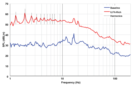
Regarding the narrow-band spectra (Figure 16) a first peak can be seen at approximately 1.3 Hz with further peaks at 1.9, 2.6, 3.2, 3.8, 4.5, 5.2, 5.9 and 9 Hz. The blade passing frequency of an IWT consists of the number of times the blades rotate past the vertical tower structure, per second. Through video footage during the ILFN-rich measurements, that number was identified and the blade passing frequency was calculated as 0.65 Hz. These peaks correspond to a harmonic series with a fundamental frequency close to 0.65 Hz, and thus constitute an integral part of the IWT acoustical signature.

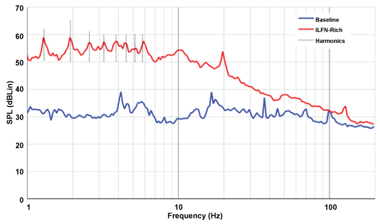
In Location 2, harmonics are not as prominent (Figure 17) as in Location 1, but peaks can still be seen at 1.3, 1.9, 2.6, 3.2, 3.9, 4.4, 5.2 and 5.9 Hz - again, acting as a signature of an IWT with a blade-pass frequency of about 0.65 Hz. An FFT of this frequency range (Figure 18) also shows these peaks.

Discussion

Large-scale public health epidemiological studies of residential ILFN contamination

Several exploratory studies have been conducted by governmental agencies [32-34] regarding the health effects of residential ILFN exposure. Many base their acoustical data on models (as per the dBA-1/3-octave methodology) rather than real, in loco, field measurements. Moreover, the unawareness of the importance of prior ILFN exposure histories when assessing health endpoints among study and control populations, predictably leads to statistically inconclusive results. As a consequence, many of the more classical groups of scientists who continue to defend the archaic notion “what you can’t hear won’t hurt you” feel justified in so doing. In the most recent French survey on the topic, results confirmed that: “wind turbines are sources of infra sounds and low-frequency sounds. However, the hearing thresholds for infra sounds and low frequencies of up to 50 Hz were not exceeded” [34]. Within the context of VAD studies, residential exposures have been investigated using the same clinical endpoints as those that were found relevant for ILFN-exposed aeronautical technicians [20-22]. These document the accelerated onset of symptoms among families exposed to residential ILFN (generated by a grain terminal [21] and by IWTs [22]) when compared to occupational exposures.

Narrow-band analysis methodology vs. dBA methodology data for IWT-generated ILFN

The benefit of narrow-band analysis becomes obvious by the identification of discrete peaks in the presence of IWT rotation, and that are absent when IWT are not rotating (Figure 17 and Figure 18). These peaks have been identified as the harmonics of a fundamental frequency, whose value precisely coincides with that of the IWT blade-pass frequency (as verified by video footage). This type of information is impossible to obtain with the dBA-1/3-octave methodology.

As many acousticians would quickly point out, the increased acoustical energy in the shed caused by rotating IWT is indistinguishable from that caused by the wind (Figure 10 vs. Figure 14 and Figure 11 vs. Figure 15). Blowing wind outside will increase the acoustical energy in the ILFN range within practically any structure (whether or not it is heard by humans). Identifying specific acoustic signatures associated with IWT operation (as demonstrated in Figure 16, Figure 17 and Figure 18), can help pin-point the contributions made by the blowing wind (structure resonance), and differentiate those from anthropogenic ILFN. But this cannot be accomplished with the dBA-1/3-octave methodology, as shown in Figure 8, Figure 9, Figure 12 and Figure 13.

Narrow-band analysis can also provide information that may in the future be relevant for dose-response values, and which the dBA-1/3-octave methodology cannot. For example, in the specific examples shown for the ILFN-rich locations (Figure 14 and Figure 15), Location 2 has similar acoustical energy at 20 Hz as Location 1. And yet, it is in Location 1 that the animal owner prefers to keep his breeding males. This may suggest that the frequencies that are more important for understanding the abnormal animal behavior (as reported by the owner) are not within the 20 Hz region.

Concomitant occupational and residential ILFN exposures in aerospace workers

In the summer of 2015, the home near the animal-sheds was abandoned by the family. IWTs had begun rotating in September 2013, and the ensuing health deterioration of family members demanded their removal. To this day, however, the property owner must return there everyday to care for the animals that are his livelihood. As in other ILFN-contaminated residences [35], this farmer's health continues to deteriorate considerably, having most recently been diagnosed with Post-Traumatic Stress Disorder.

Aerospace workers who are exposed to occupational ILFN greatly benefit from the recovery periods encountered in their homes (presumably absent of anthropogenic ILFN) [16,19,36]. A growing segment of the world population, however, particularly from rural and suburban areas, has been confronted with ILFN-contamination in their homes. Some of these families include aerospace professionals (and other occupationally exposed ILFN workers), who are now exposed to ILFN both at work and at home.

The ongoing citizen-based research effort into ILFN-induced pathology to which these authors contribute [30] includes providing proper acoustical evaluations to participating citizens’ properties, and also providing pertinent medical diagnostic tests, including the established VAD diagnostic tests [16,21,37]. Within this context, initial steps include obtaining personal and medical histories from each participating citizen. Histories are obtained through one-on-one interviews that can last over 2 hours. Some of the citizens already interviewed include aerospace workers who are (or were) occupationally exposed to ILFN environments. Of these, some were already sleeping in ILFN-rich homes (due to anthropogenic sources), while others were expected to have sources of anthropogenic ILFN constructed near (< 3 km) their residential areas. Clinical information revealed in the interviews and corroborated by accompanying medical documentation, has been reiterating the association between symptom gravity and overall ILFN exposure.

People exposed to ILFN at work and at home see an acceleration of the onset of ILFN-induced pathology when compared to individuals who ‘only’ have ILFN exposure at work (assuming similar fetal, childhood and adolescent ILFN exposures). Individuals who are only exposed to ILFN-rich environments in the home see an accelerated onset of symptoms when compared to those who are only exposed to occupational ILFN-rich environments [20-22]. The reasons for this are twofold: on the one hand, when ILFN-exposed workers leave their place of employment, they undergo a biological respite from the agent of disease; on the other hand, ILFN-rich environments in the home are usually synonymous with sleeping in an anthropogenic ILFN-rich environment. Biological processes that only occur during sleep time are now occurring in the presence of an agent of disease [38].

Limitations of this study

When laboratorial studies are conducted using airborne acoustical phenomena, environmental parameters can be controlled with more or less ease. In real environments, however, an acoustic environment will not be homogeneous over any significant area or any significant time. Outdoors the environment may be reasonably homogeneous over tens of meters (apart from the interference effects from multiple sound sources creating ‘heightened noise zones’ possibly only a few meters across [39]). However, indoor environments can vary significantly over distances less than a meter. Furthermore, the acoustical differences between the two locations may have been due to time-wise changes between recording times.

Conclusions

This report highlights the difference in acoustical information gathered with two distinct methods of analysis: one sanctioned by current legislation and guidelines, and focused on protecting hearing impairment (dBA-1/3-octave methodology); the other, sanctioned by the bio-physical sciences and focused on protecting whole-body health (narrow-band methodology). The latter provides important information on the temporal and frequency profiles that are crucial for understanding how ILFN affects human health (considering both immediate and long-term effects).

The archaic notion of “what you can’t hear won’t hurt you” is reflected in the dBA-1/3-octave methodology, i.e., the hearing sensory pathway is the only one through which ILFN can adversely affect humans. This position is incompatible with the Scientific Method and with evidence-based medicine when quantifying a potential agent of disease, such as ILFN.

The clinical evolution of ILFN-induced pathology greatly depends on exposure-time patterns. Individuals, who work in ILFN-rich environments and simultaneously live in ILFN-rich homes, may see an accelerated onset of specific symptoms when compared with individuals who only live in the ILFN-rich home, with no prior or current history of occupational ILFN exposure. Therefore, the increasing number of ILFN-rich acoustic environments within rural residential dwellings poses a serious problem for ILFN-exposed aerospace workers, as their biological recovery periods (that occur when away from the ILFN-rich environment) may be greatly reduced, or even become non-existent.

In order to protect populations from excessive and harmful ILFN exposure, serious epidemiological studies under the auspices of ‘Public Health’ must be undertaken. An important step in that direction is taken here, showing the importance of departure from the established guidelines and legislation in order to obtain a scientifically useful quantification of the agent of disease under scrutiny.

Acknowledgements

The authors would like to thank Mr. Kaj Bank Olesen for allowing acoustical measurements on his property, and also Mr. Boye Janssen for acquiring all relevant DMI weather information. The authors also thank Mr. Finn Nielsen for all logistical support in Denmark.

Financial Disclosure

Due to his efforts in the creation of the SAM Scribe system, author HHCB has a financial interest in the SAM Scribe system.

Disclaimer

The authors of this paper:

1) Do not harbor anti-technology sentiments;

2) Consider industrial activities to be important to modern technological societies;

3) Have scrutinized the data under one and only on agenda - pure scientific inquiry;

4) Are not producing a report arguing against industrial complexes;

5) Are not producing an environmental noise assessment report focused on wind turbines;

6) Provided all acoustical evaluations and analyses pro bono.

References

1. World Health Organization (2011) Burden of disease from environmental noise.
2. World Health Organization (1999) Guidelines for community noise. In: Berglund B, Lindvall T, Schwela DH, World Health Organization, Geneva.
3. World Health Organization (2016) International Classification of Diseases. ICD-10 Version 2016.
4. Ingber DE (1993) Cellular tensegrity: defining new rules of biological design that governs the cytoskeleton. J Cell Sci 104: 613-627.
5. Ingber DE (2003) Mechanobiology and diseases of mechanotransduction. Ann Med 35: 564-577.
6. Ingber DE (2004) Mechanochemical basis of cell and tissue regulation. Mech Chem Biosyst 1: 53-68.
7. Motro R (2003) Tensegrity - Structural systems for the future. Hermes Science Publishing Limited, London, UK.
8. Sun Z, Guo SS, Fässler R (2016) Integrin-mediated mechanotransduction. J Cell Biol 216: 445-456.
9. Xu GK, Li B, Feng XQ, et al. (2016) A tensegrity model of cell reorientation on cyclically stretched substrates. Biophys J 111: 1478-1486.
10. Castelo Branco NA, Águas AP, Sousa Pereira A, et al. (1999) The human pericardium in vibroacoustic disease. Aviat Sp Environ Med 70: 54-62.
11. Castelo Branco NA, Gomes-Ferreira P, Monteiro E, et al. (2003) Respiratory epithelia in Wistar rats after 48 hours of continuous exposure to low frequency noise. Rev Port Pneumol 9: 473-479.
12. Alves-Pereira M, Joanaz de Melo J, Castelo Branco NAA (2005) Pericardial biomechanical adaptation to low frequency noise stress. In: A Méndez-Vilas, Recent Advances in Multidisciplicnary Applied Physics. Elsevier, London, UK, 363-367.
13. Ponomar’kov VI, Tysik Ayu, Kudryavtseva VI, et al. (1969) Biological action of intense wide-band noise on animals. In: Problems of Space Biology. NASA TT F-529, 307-309.
14. Nekhoroshev AS, Glinchikov VV (1992) Morphological research on the liver structures of experimental animals under the action of infrasound. Aviakosm Ekolog Med 26: 56-59.
15. Nekhoroshev AS, Glinchikov VV (1991) Effect of infrasound on morphofunctional changes in myocardium exposed to infrasound. Gig Sanit 12: 56-58.
16. Castelo Branco NAA (1999) Clinical stages of vibroacoustic disese. Aviat Space Environ Med 70: 32-39.
17. Castelo Branco NA, Alves-Pereira M (1999) Vibroacoustic disease. Aviat Space Environ Med 70: 1-153.
18. Castelo Branco NA, Alves-Pereira M (2004) Vibroacoustic disease. Noise Health 6: 3-20.
19. Alves-Pereira M, Castelo Branco NAA (2007) Vibroacoustic disease: Biological effects of infrasound and low frequency noise explained by mechanotransduction cellular signaling. Prog Biophys Mol Biol 93: 256-279.
20. Torres R, Tirado G, Roman A, et al. (2001) Vibroacoustic disease induced by long-term exposure to sonic booms. Proceedings Internoise 2001, The Hague, Holland, 1095-1098.
21. Araujo A, Alves-Pereira M, Joanaz de Melo J, et al. (2004) Vibroacoustic disease in a ten-year-old male. Proceedings Internoise 2004, Prague, Czech Republic.
22. Alves-Pereira M, Castelo Branco NAA (2007) In-home wind turbine noise is conducive to vibroacoustic disease. Wind Turbine Noise, Lyon, France.
23. Alves-Pereira M, Joanaz de Melo J, Castelo Branco NAA (2005) Actin- and tubulin-based structures under low frequency noise stress. In: A Méndez-Vilas, Recent Advances in Multidisciplinary Applied Physics. Elsevier, London, UK, 955-979.
24. Alves-Pereira M, Joanaz de Melo J, Castelo Branco NAA (2005) Low frequency noise exposure and biological tissue: reinforcement of structural integrity? In: A Méndez-Vilas, Recent Advances in Multidisciplinary Applied Physics. Elsevier, London, UK, 961-966.
25. Cooper S (2014) The Results of an Acoustic Testing Program Cape Bridgewater Wind Farm. Energy Pacific (Vic) Pty Ltd, Melbourne, Australia.
26. Cooper S (2015) Soundscape of a wind farm, Cape Bridgewater experience. Proceedings of the 170th Meeting of the Acoustical Society of America, Jacksonville, FL, USA.
27. www.smart-technologies.co.nz
28. Bakker H, Rapley B, Summers R, et al. (2017) An affordable recording instrument for the acoustical characterisation of human environments. Proceedings International Conference Biological Effects of Noise, Zurich, Switzerland.
29. http://www.primo.com.sg/japan-low-freq-micro
30. Bakker HHC, Alves-Pereira M, Summers SR (2017) Citizen Science Initiative: Acoustical Characterisation of Human Environments. Proceedings International Conference Biological Effects of Noise, Zurich, Switzerland.
31. http://vindinfo.dk/english.aspx
32. Health Canada (2014) Wind turbine noise and health study.
33. National Health and Medical Research Council of Australia (2013) Systematic review of the human health effects of wind farms.
34. French Agency for Food, Environmental and Occupational Health & Safety (ANSES) (2017) Exposure to low-frequency sound and infrasounds from wind farms: improving information for local residents and monitoring noise exposure.
35. Castelo Branco NA, Alves-Pereira M, Martinho Pimenta A, et al. (2015) Low frequency noise-induced pathology: contributions provided by the Portuguese wind turbine case. Euronoise 2015, Maastricht, The Netherlands.
36. Castelo Branco NA, Rodriguez E, Alves-Pereira M, et al. (1999) Vibroacoustic disease: some forensic aspects. Aviat Sp Environ Med 70: 145-151.
37. Castelo Branco NA, Alves-Pereira M, Martinho Pimenta A, et al. (2015) Clinical protocol for evaluating pathology induced by low frequency noise exposure.
38. Nissenbaum MA, Aramini JJ, Hanning CD (2012) Effects of industrial wind turbine noise on sleep and health. Noise Health 14: 237-243.
39. Rapley BI, Bakker HHC (2010) Sound, Noise, Flicker and the Human Perception of Wind Farm Activity. In: Atkinson, Rapley Consulting, Palmerston North, New Zealand, 235-236.
40. https://commons.wikimedia.org/wiki/File:Acoustic_weighting_curves_(1).svg
41. Dirac Delta Science & Engineering Encyclopedia (2017) G-weighted overall level.
42. Dirac Delta Science & Engineering Encyclopedia (2017) A-Weighting.
43. https://www.fhwa.dot.gov/environment/noise/regulations_and_guidance/ analysis_and_abatement_guidance/polguide01.cfm
44. Bento Coelho JL, Ferreira A, Serrano J, et al. (1999) Noise assessment during aircraft run-up procedures. Aviat Space Environ Med 70: 22-26.
45. Bento Coelho JL, Ferreira A, Serrano J, et al. (1994) Noise exposure in the aeronautical industry. Internoise 31: 741-744.