Omni-Joint a Comparative Study for Singularity

Abstract

Robots and mechanical systems mainly consist of links and joints, hence studying different joints and coming up with new joints will contribute in advancing them.

The scope of this paper is to find the singularity of an Ordinary 2 Dof joint, a Hooke's (or Universal) joint, and the Omni-Joint. The methodology used in this paper is; finding the singularity case using the determinant of the Jacobian (which transforms from the joint-space to the work-space) using MATLAB. The determinant is plotted; first with respect to the variables of the joint-space, second with respect to the variables of the work-space.

The results are that Omni-Joint has only one singularity, which is at a deviation angle of 180 degrees. The Ordinary joint suffers from two singularities at different deviation angels; one at 0° (which is in the range of the field of motion), and one at 180°. The Hooke's joint suffer from two singularities at two postures, both at deviation angel of 90° (which are in the range of field of motion), and discontinuity in its range of field of motion.

Keywords

Joint, Omni joint, Omni-joint mechanism design, Hook, Hooke, Universal U joint, Wrist joint, RR, 2 DoF, Kinematic singularity

Introduction

Researchers have studied the kinematics of several joints including universal and joints used for couplings such as the work of Shah and Patil, [1], and Williams [2]. Studying the singularities have taken researchers interest for decades and was reported by Williams II [3]. They used different analytical methods and simulation models Arora [4], Jawale and Thorat [5]. Others have tried to control joints motion to overcome singularity problems associated with those types of joints such as the work of Han and Park [6]. Applications of universal joints and 3 UPU manipulators have been reported by Binbin, Zengming, and Kai [7].

The study of omnidirectional manipulators has been conducted for kinematics, modeling, and simulation for using those joints in autonomous mobile robots Sillas, Hurtado, Vargas, Resendiz, and Tovar [8], Djebrani, Benali, and Abdessemed [9].

Ongoing research is being reported for the design of parallel universal joints using deterministic approaches such as the work of Yan, Yu and Zhao [10] or by approximate methods such as finite element Cheng, Wang, Yang and Yang [11].

Design and kinematic analysis are also being reported in the literature as an active field of research Pan, Chen, Kang and Wang [12]; Lin, Wang, Zhang and Jiang, [13].

The Omni-Joint is a mechanical joint composed of two symmetrical halves. It can move in any direction at any instant on a wide range of motion and works as a constant velocity flexible coupling with a deviation angle greater than 90°. It is only has one singularity posture, if the deviation angle is 180°. The Ordinary 2 DoF joint and the Hooke's joint are commonly used for robotic joints.

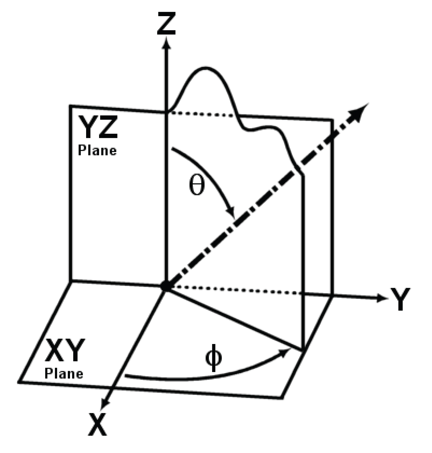
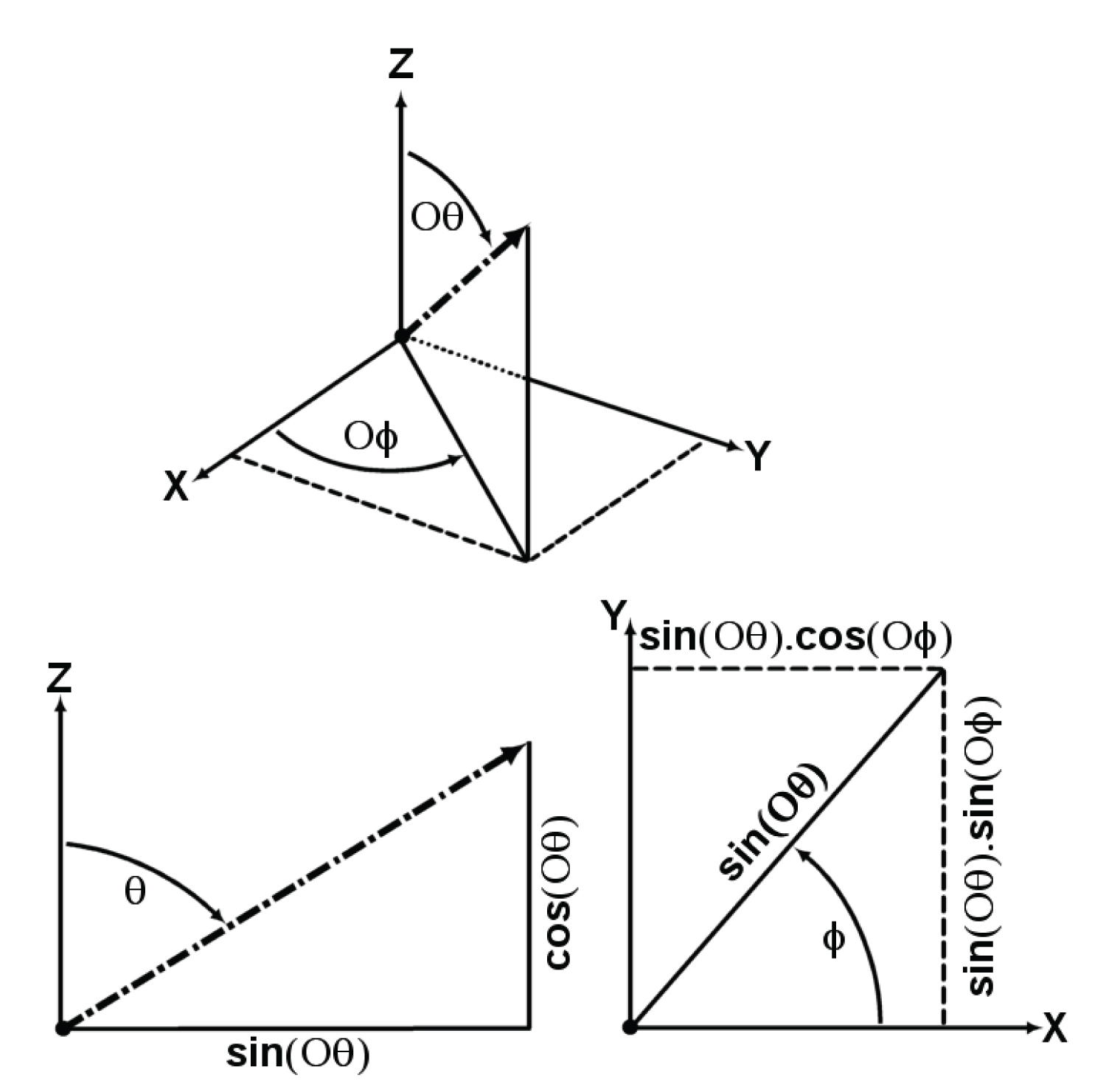
The coordinate system used for the work-space in this paper is the spherical coordinate system, θ is deviation angle, φ is the azimuth angle as shown in Figure 1.

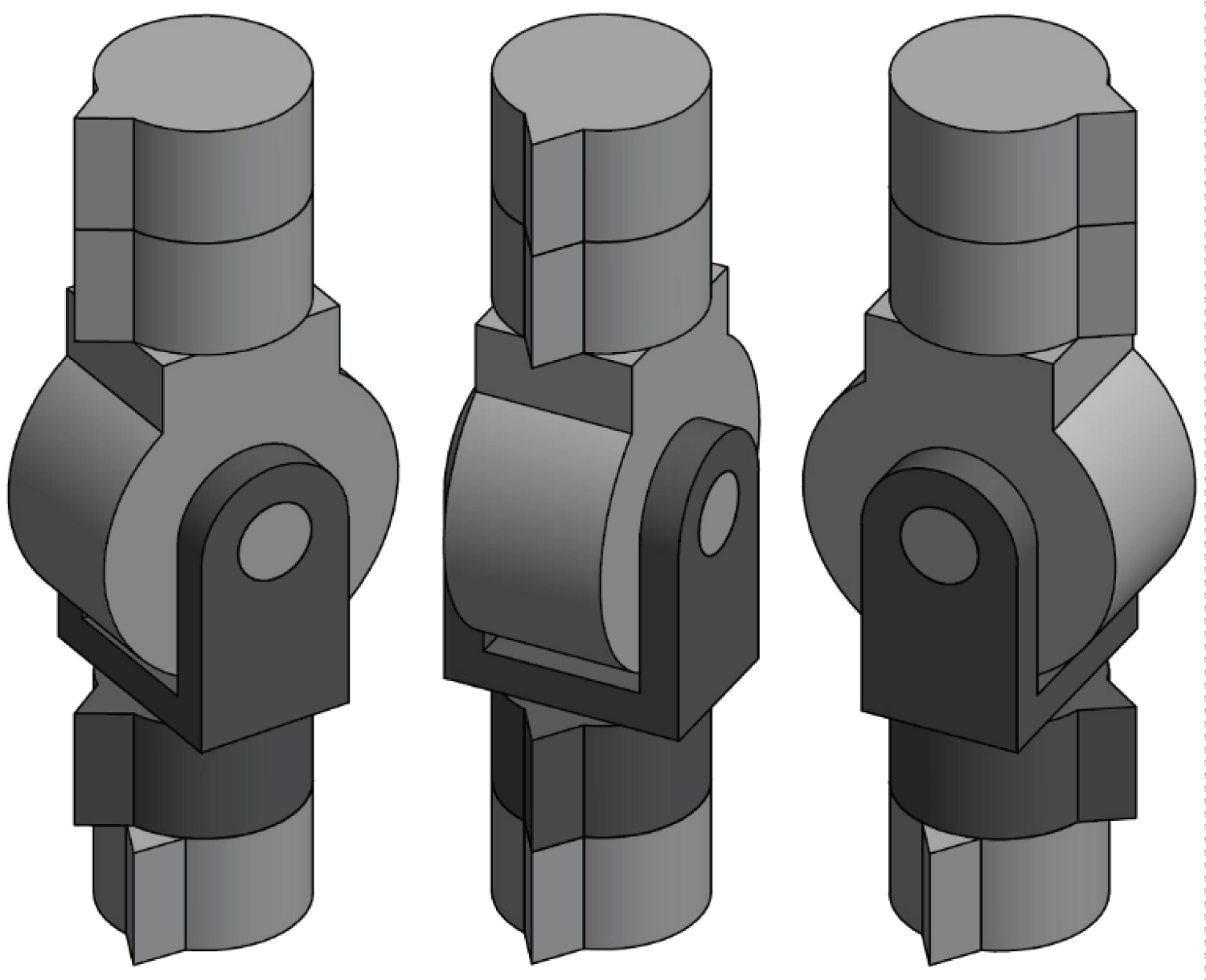
The Omni-Joint has three Configurations:

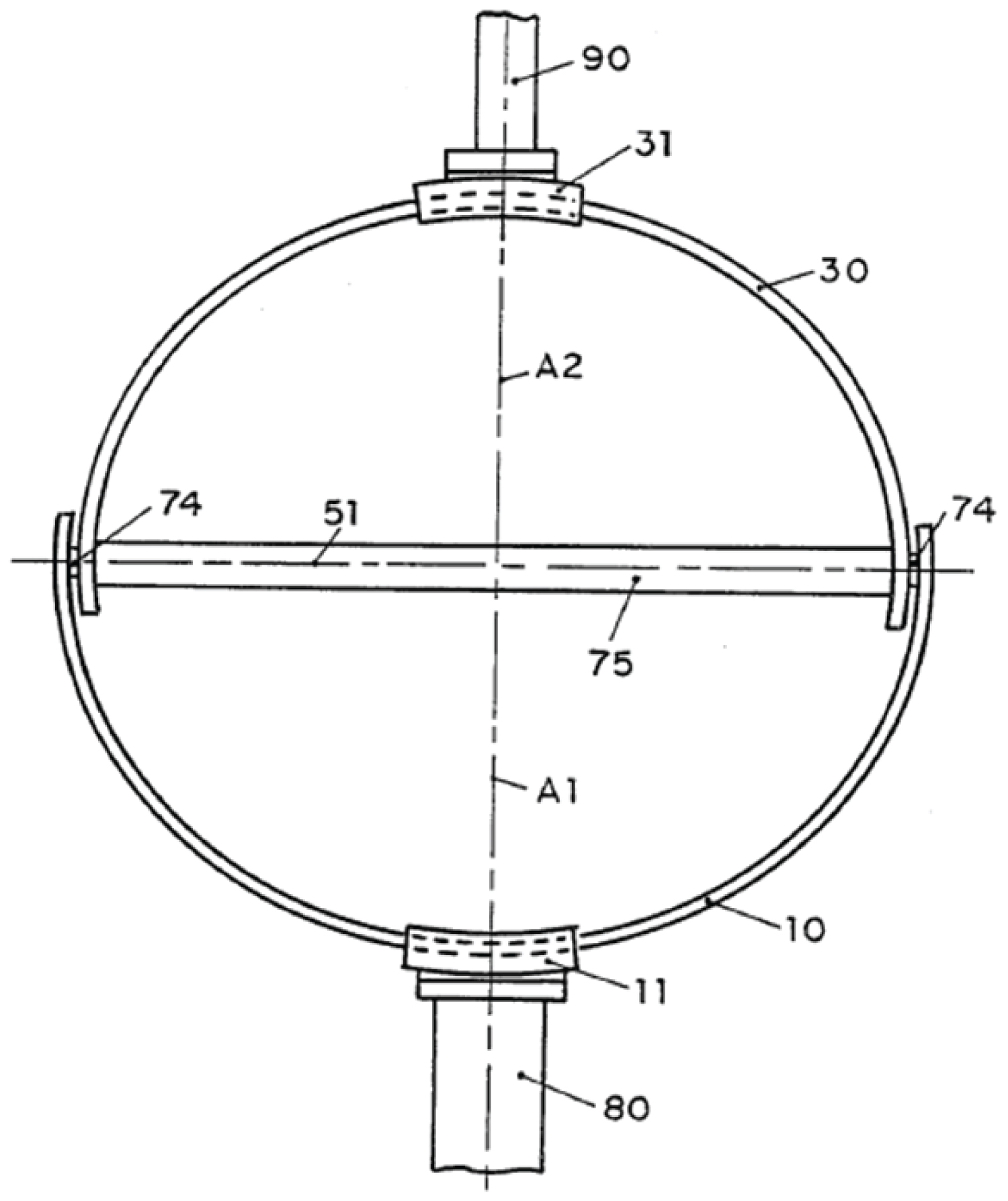
Configuration-II was first introduced by Duta, Opera, and Stanisic [14]. It only has one pair of arcs with only one hinge as shown in Figure 2.

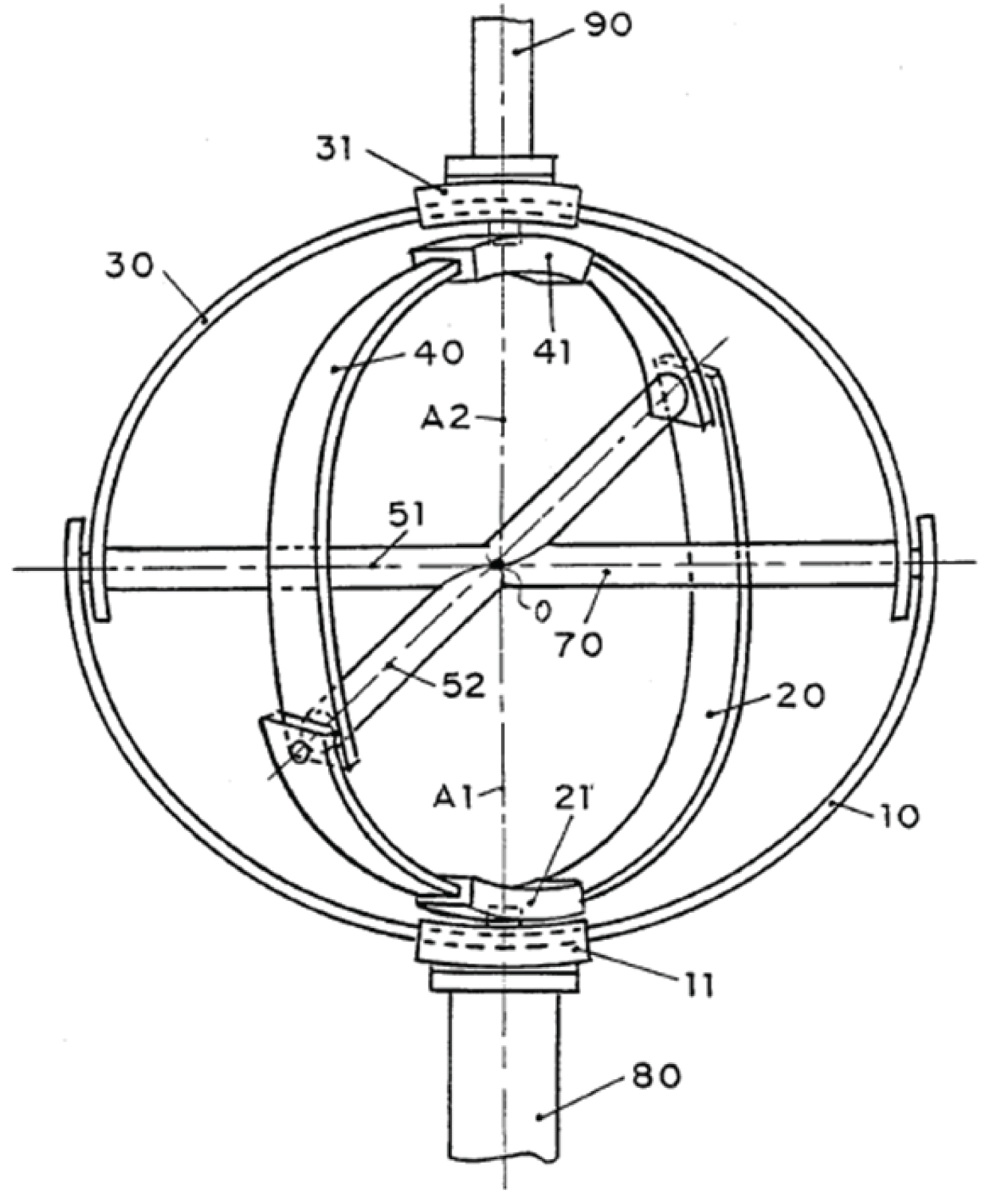
Configuration-III was also first introduced by Duta, Opera, and Stanisic [14]. It has two pairs of arcs. The angle between the hinges connecting the arc parts is always 90 degrees as shown in Figure 3.

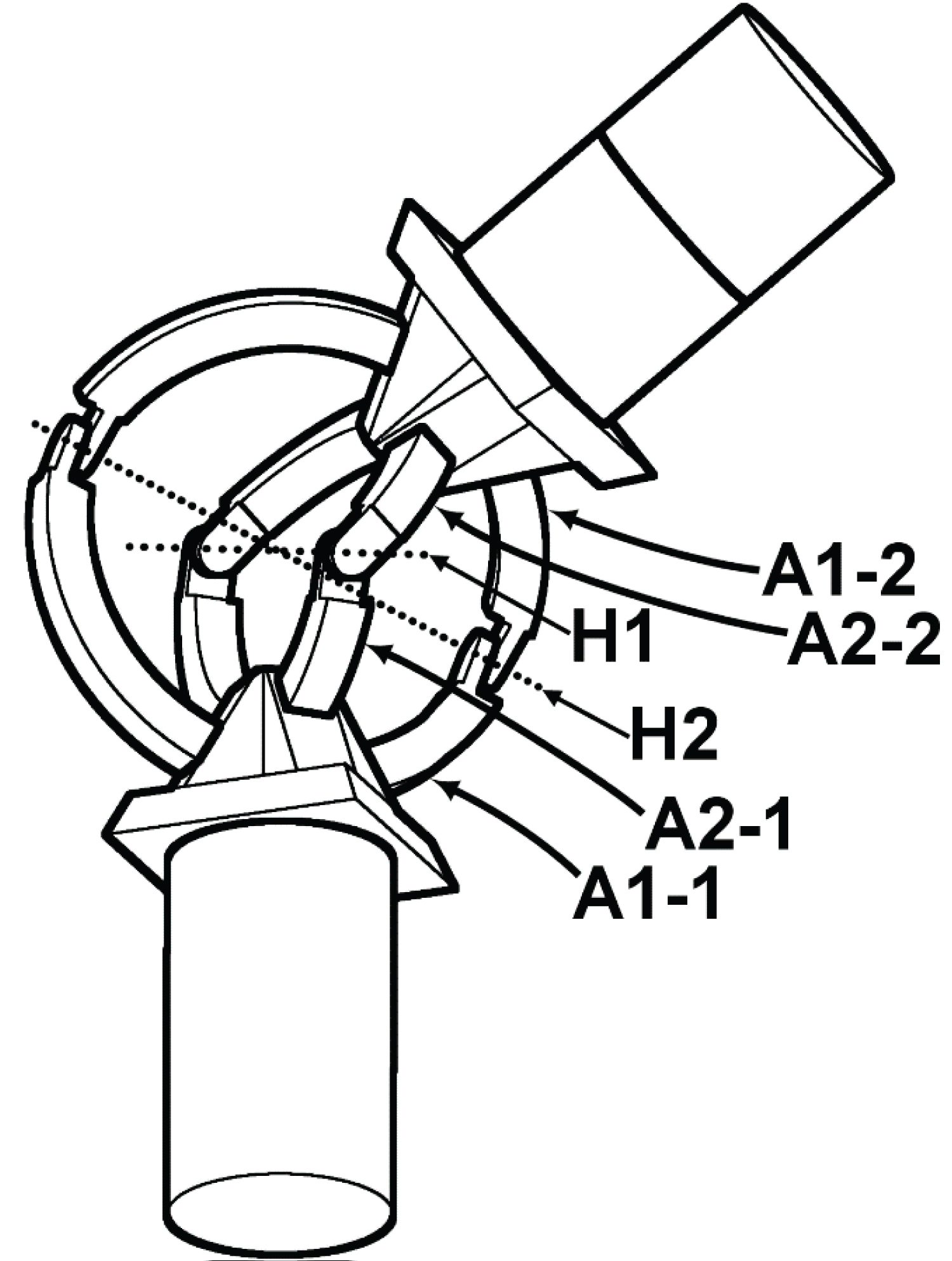
Omni-Joint Configuration-I was first introduced by AboZaied and El Saeid [15]. It has two pairs of arcs (A1-1 & A1-2, and A2-1 & A2-2). The angle between the hinges (H1 and H2) connecting the arc parts is variable as shown in Figure 4.

Note that, for the Omni-Joint Configuration-I there exist four combinations of degrees of freedom to be controlled:

• The angles of both the arcs, as shown in Figure 5, which is the focus of this paper.

• The angle of an arc of one of the pairs, and the hinge connecting this pair.

• The angle of an arc of one of the other pairs, and the hinge connecting this pair.

• The angles of both hinges.

For the Omni-Joint Configuration-II there exists one combination of degrees of freedom to be controlled:

• The angle of an arc, and the hinge connecting this pair.

For the Omni-Joint Configuration-III there exist four combinations of degrees of freedom to be controlled:

• The angles of both the arcs.

• The angle of an arc of one of the pairs, and the hinge connecting this pair.

• The angle of an arc of one of the other pairs, and the hinge connecting this pair.

• The angles of both hinges.

Methodology and Procedure

Omni-Joint Configuration-I

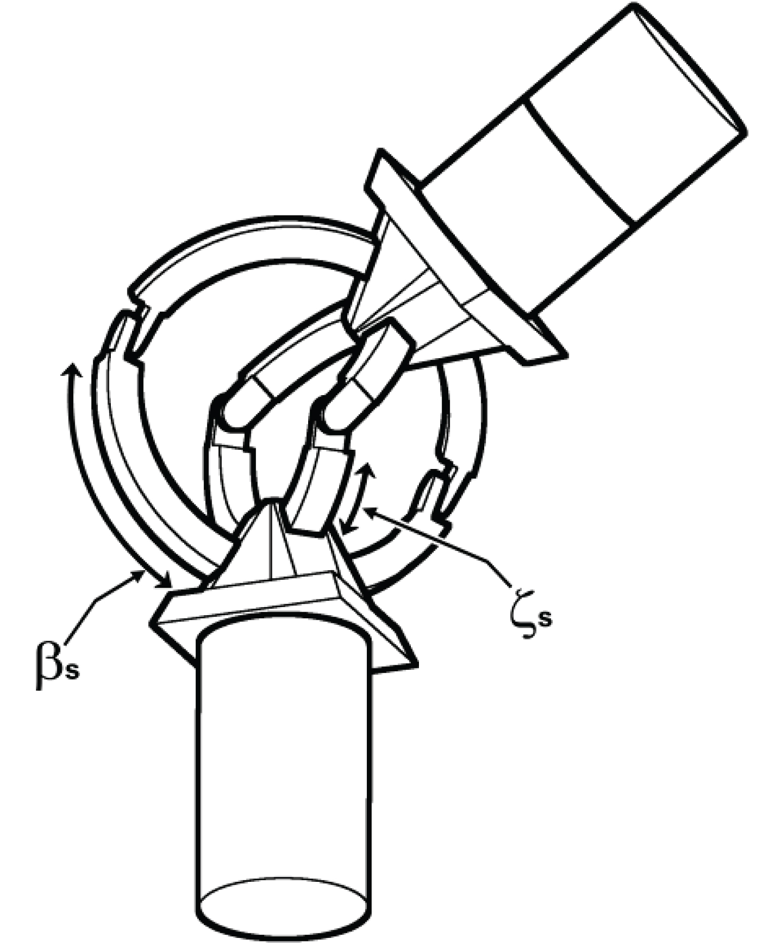
1) Forward and Inverse Kinematics Equations: Figure 5 shows the shape of the Omni-Joint Configuration-I. With two degrees of freedom; βs and ζs, for pointing the joint in space.

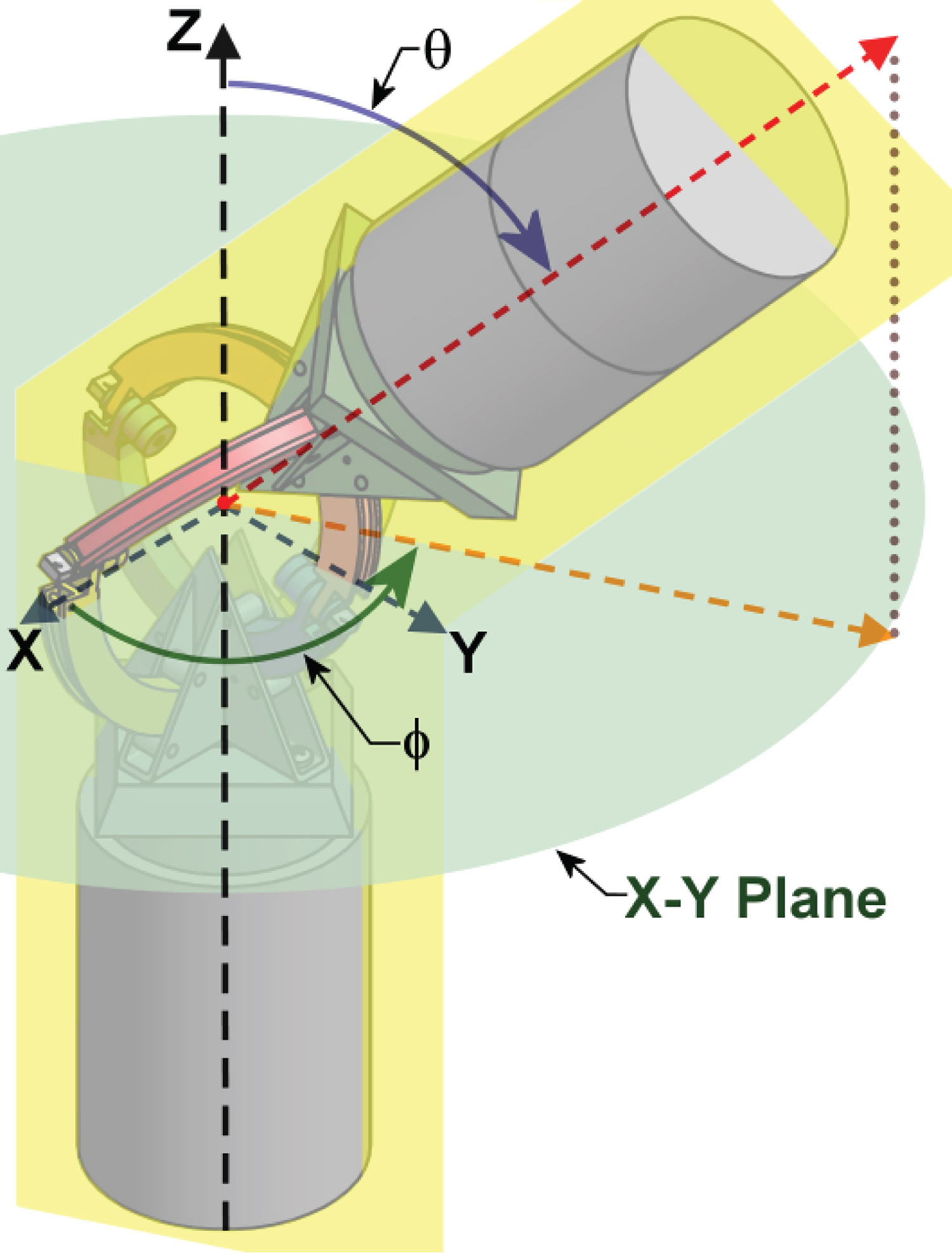
Figure 6 shows the Omni-Joint Configuration-I, with the coordinates of the world-space θ & φ.

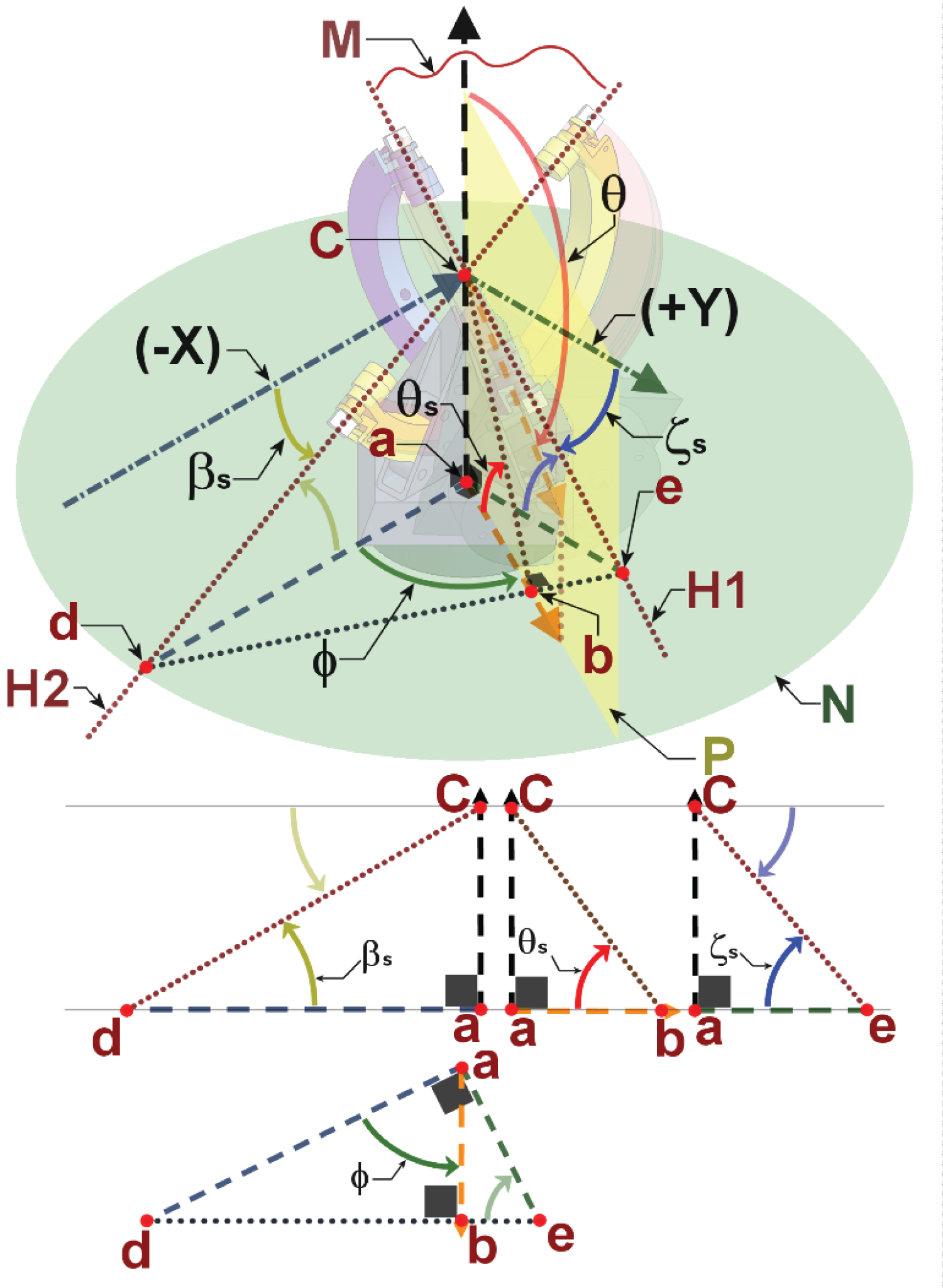
Figure 7 shows the Omni-Joint bent. It also shows the relative positions of work-space variables; θ and φ, and the joint-space variables βs and ζs. Configuration-I of Omni joint is not an open chain mechanism; hence D-H table is not used to find the forward kinematics. Instead a geometrical method is used. Plane N is parallel to the X-Y plane and exist any place along the Z-axis below of origin point C. Plane P is the plane where the deviation angle θ is measured. Plane M is formed by the hinges H1 and H2 of both arc pairs. Hence plane M is a mirror plane, where both halves of the joint are symmetrical about. This means that when plane M inclines, it forms an angle θs with the plane N, which is half the value of θ. This is due to the fact that the angle that lies between any two planes is equal to the angle formed by the two normal to these planes. The distance between the center point C and plane N is taken to be (aC). The value of (aC) is arbitrary as the location of plane N is along the Z-axis is irrelevant. Regardless of the value of (aC), the relations between all the angles remain intact. The value of (aC) is used to derive the mathematical equations, upon derivation the variable of (aC) is cancelled out automatically. This is the same for all the distances shown in Figure 7. Angle βs is measured in the counterclockwise direction about the Y-axis. Angle ζs is measured in the clockwise direction about the X-axis.

Forward kinematics:

As mentioned:

$${\theta }_s=\frac{1}{2}\theta \left(1.1\right)$$

From the geometry:

$$\tan ({\theta }_s)=\frac{\overline{ac}}{\overline{ab}}\left(1.2\right)$$

From the triangle $\Delta aCd:$ $$\overline{ad}=\frac{\overline{ac}}{\tan \left({\beta }_s\right)}\left(1.3\right)$$

From the triangle $\Delta aCe:$ $$\overline{ae}=\frac{\overline{aC}}{\tan \left({\zeta }_s\right)}\left(1.4\right)$$

From the triangle $\Delta ade$ and applying Pythagoras:

$$\overline{de}=\sqrt{{\overline{ad}}^2+{\overline{ae}}^2}$$

Substituting eqn.1.3 and eqn.1.4 in the previous equation

$$\overline{de}=\sqrt{{\left(\frac{\overline{aC}}{\tan \left({\beta }_s\right)}\right)}^2+{\left(\frac{\overline{aC}}{\tan \left({\zeta }_s\right)}\right)}^2}\left(1.5\right)$$

From the triangle $\Delta ade$ and the concept of triangles similarity:

$$\frac{\overline{ab}}{\overline{ae}}=\frac{\overline{ad}}{\overline{de}}$$

Substituting eqn.1.3 and eqn.1.4 in the previous equation

$$\overline{ab}={\frac{{\overline{C}}^2}{\overline{de.}\tan \left({\beta }_s\right).\tan \left({\zeta }_{{}_s}\right)}}^{}\left(1.6\right)$$

Substituting eqn.1.6 in eqn.1.2

$$\tan ({\theta }_s)=\frac{\overline{aC}.\overline{de}.\tan \left({\beta }_s\right).\tan ({\zeta }_s)}{\overline{a{c}^2}}$$

Substituting eqn.1.5 in the previous equation

$$\tan ({\theta }_s)=\frac{\tan \left({\beta }_s\right).\tan \left({\zeta }_s\right)}{\overline{a{c}^2}}.\sqrt{{\left(\frac{\overline{aC}}{\tan \left({\beta }_s\right)}\right)}^2+{\left(\frac{\overline{aC}}{\tan \left({\zeta }_s\right)}\right)}^2}$$

Substituting eqn.1.1 in the previous equation and simplifying

$$\tan \left(\theta /2\right)=\sqrt{{\tan }^2\left({\beta }_s\right)+{\tan }^2\left({\zeta }_{{}_s}\right)}\left(1.7\right)$$

$$\theta =2{\tan }^{-1}\left(\sqrt{{\tan }^2\left({\beta }_s\right)+{\tan }^2\left({\zeta }_s\right)}\right)\left(1.8\right)$$

From the triangle $\Delta ade:$

$$\sin \left(\varphi \right)=\frac{\overline{ab}}{\overline{ae}}$$

Substituting eqn.1.2 and eqn.1.4 in the previous equation

$$\sin \left(\varphi \right)=\frac{\tan \left({\zeta }_s\right)}{\tan \left({\theta }_s\right)}\left(1.9\right)$$

From the triangle $\Delta ade$:

$$\cos \left(\varphi \right)=\frac{\overline{ab}}{\overline{ad}}$$

Substituting eqn.1.2 and eqn.1.3 in the previous equation

$$\cos \left(\varphi \right)=\frac{\tan \left({\beta }_s\right)}{\tan \left({\theta }_s\right)}\left(1.10\right)$$

From eqn.1.9 and eqn.1.10:

$$\tan \left(\varphi \right)=\frac{\tan \left({\zeta }_s\right)}{\tan \left({\beta }_s\right)}\left(1.11\right)$$

$$\varphi ={\tan }^{-1}\left(\frac{\left(\tan \left({\zeta }_s\right)\right)}{\left(\tan \left({\beta }_s\right)\right)}\right)\left(1.12\right)$$

From eqn.1.8 and eqn.1.12, we get the forward kinematics equation:

$$\left\{\begin{array}{l}\theta =2{\tan }^{-1}\left(\sqrt{{\tan }^2\left({\beta }_s\right)+{\tan }^2\left({\zeta }_s\right)}\right)\\ \varphi ={\tan }^{-1}\left(\frac{\left(\tan \left({\zeta }_s\right)\right)}{\left(\tan \left({\beta }_s\right)\right)}\right)\end{array}\right\}\left(1\right)$$

Inverse kinematics:

From the geometry:

$$\begin{array}{l}\tan \left({\beta }_s\right)=\frac{\overline{ac}}{\overline{ad}}\\ \tan \left({\beta }_s\right)=\frac{\overline{aC}}{\overline{ad}}.\frac{\overline{ab}}{\overline{ab}}=\frac{\overline{aC}}{\overline{ab}}.\frac{\overline{ab}}{\overline{ad}}\end{array}$$

Taking into consideration that:

$$\tan \left({\theta }_s\right)=\frac{\overline{aC}}{\overline{ab}}and\cos \left(\varphi \right)=\frac{\overline{ab}}{\overline{ad}}$$

$$\tan \left({\beta }_s\right)=\tan \left({\theta }_s\right).\cos \left(\varphi \right)\left(2.1\right)$$

$${\beta }_s={\tan }^{-1}\left(\tan \left({\theta }_s\right).\cos \left(\varphi \right)\right)\left(2.2\right)$$

From the geometry:

$$\tan \left({\zeta }_s\right)=\frac{\overline{aC}}{\overline{ae}}$$

$$\tan \left({\zeta }_s\right)=\frac{\overline{aC}}{\overline{ae}}.\frac{\overline{ab}}{\overline{ab}}=\frac{\overline{aC}}{\overline{ab}}.\frac{\overline{ab}}{\overline{ae}}$$

Taking into consideration that:

$$\tan \left({\theta }_s\right)=\frac{\overline{aC}}{\overline{ae}}and\sin \left(\varphi \right)=\frac{\overline{ab}}{\overline{ae}}$$

$$\tan \left({\zeta }_s\right)=\tan \left({\theta }_s\right).\sin \left(\varphi \right)\left(2.3\right)$$

$${\zeta }_s={\tan }^{-1}\left(\tan \left({\theta }_s\right).\sin \left(\varphi \right)\right)\left(2.4\right)$$

From eqn.2.2 and eqn.2.4, we get the inverse kinematics equation:

$$\left\{\begin{array}{l}{\beta }_s={\tan }^{-1}\left(\tan \left({\theta }_s\right).\cos \left(\varphi \right)\right)\\ {\zeta }_s={\tan }^{-1}\left(\tan \left({\theta }_s\right).\sin \left(\varphi \right)\right)\end{array}\right\}\left(2\right)$$

2) Derivation of the Jacobian J:

$$\left[\stackrel{.}{{}_{\stackrel{.}{\varphi }}^{\theta }}\right]=J\left[{}_{\stackrel{.}{{\zeta }_S}}^{\stackrel{.}{{\beta }_S}}\right]$$

$$J=\left[\begin{array}{l}\frac{\partial \theta }{\partial {\beta }_S}\frac{\partial \theta }{\partial {\zeta }_S}\\ \frac{\partial \varphi }{\partial {\beta }_S}\frac{\partial \varphi }{\partial {\zeta }_S}\end{array}\right]$$

Using MATLAB;

$$\frac{\partial \theta }{\partial {\beta }_s}=\frac{2\tan \left({\beta }_s\right)\left({\tan }^2\left({\beta }_s\right)+1\right)}{\left({\tan }^2\left({\beta }_s\right)+{\tan }^2\left({\zeta }_s\right)+1\right)\sqrt{\tan \left({\beta }_s\right)+{\tan }^2}\left({\zeta }_s\right)}$$

$$\frac{\partial \theta }{\partial {\zeta }_s}=\frac{2\tan \left({\zeta }_s\right)\left({\tan }^2\left({\zeta }_s\right)+1\right)}{\left({\tan }^2\left({\beta }_s\right)+{\tan }^2\left({\zeta }_s\right)+1\right)\sqrt{{\tan }^2\left({\beta }_s\right)+{\tan }^2}\left({\zeta }_s\right)}$$

$$\frac{\partial \varphi }{\partial {\beta }_s}=\frac{-\tan \left({\zeta }_s\right)\left({\tan }^2\left({\beta }_s\right)+1\right)}{{\tan }^2\left({\beta }_s\right)+{\tan }^2\left({\zeta }_s\right)}$$

$$\frac{\partial \varphi }{\partial {\zeta }_s}=\frac{-\tan \left({\zeta }_s\right)\left({\tan }^2\left({\beta }_s\right)+1\right)}{{\tan }^2\left({\beta }_s\right)+{\tan }^2\left({\zeta }_s\right)}$$

3) Derivation of the Determinant with respect to βs &ζs.

Using MATLAB;

$$d=\frac{2\left({\tan }^2\left({\beta }_s\right)+1\right)\left({\tan }^2\left({\zeta }_s\right)+1\right)}{\left({\tan }^2({\beta }_s\right)+{\tan }^2\left({\zeta }_s\right)+1\sqrt{{\tan }^2\left({\beta }_s\right)+{\tan }^2\left({\zeta }_s\right)}}\left(3\right)$$

4) Derivation of the Determinant with respect to θ & φ:

Substituting (2) in (3) to get the Determinant with respect to θ and φ. By using MATLAB (4) is derived;

$$D=\frac{2\left({\tan }^2\left(\frac{\theta }{2}\right){\cos }^2\left(\varphi \right)+1\right)\left({\tan }^2\left(\frac{\theta }{2}\right){\sin }^2\left(\varphi \right)+1\right)\left(\frac{\cos \left(\theta \right)+1}{2}\right)}{\sqrt{\frac{-\cos \left(\theta \right)+1}{\cos \left(\theta \right)+1}}}\left(4\right)$$

5) Plotting Determinant (3) with βs and ζs using MATLAB:

Figure 3 shows the Determinant as a function in βs and ζs, where βs varies from -90° to +90°, and ζs from -90° to +90°.

6) Finding the limits at the borders of the surface:

The points at the borders of the surface are undefined, where βs = -90°, βs = +90°, ζs = - 90°, and ζs = +90°. MATLAB is used to find the limits at these borders (Applying L'Hospital's Rule twice).

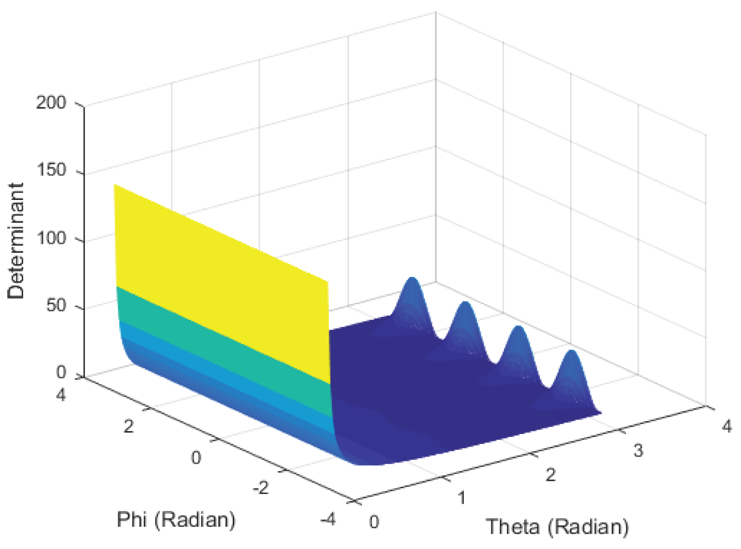
7) Plotting Determinant (4) with θ and φ using MATLAB:

Figure 4 shows the Determinant as a function in θ and φ, where θ varies from 0° to +180°, and φ from -180° to +180°.

Ordinary Joint

1) Forward Kinematics Equation:

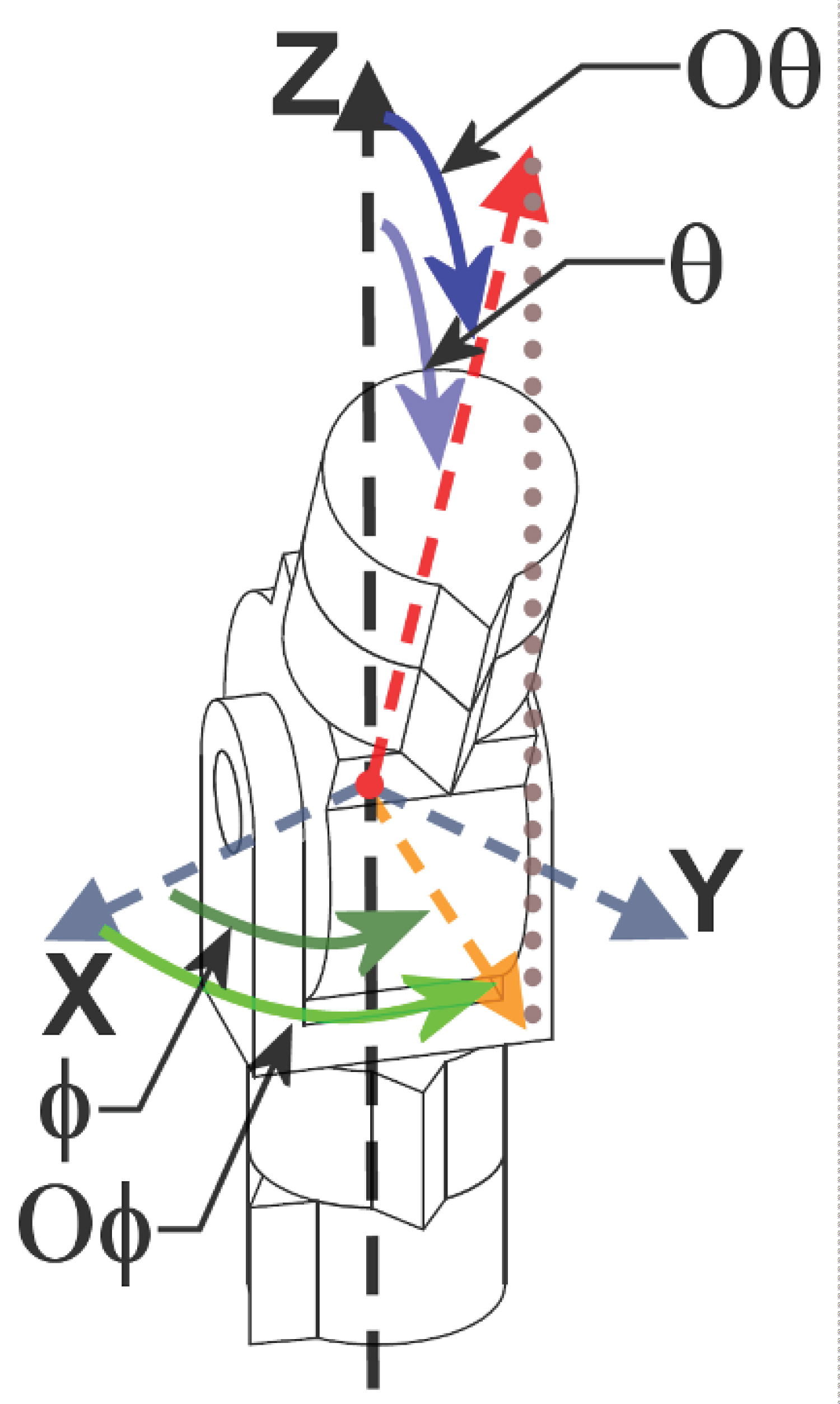
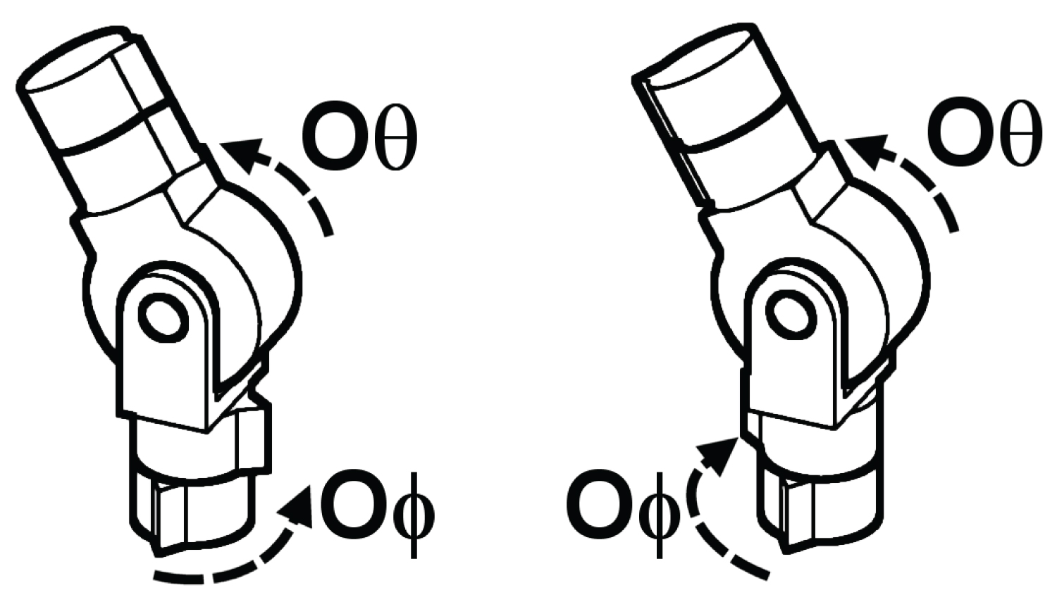
Figure 8 shows the shape of the Ordinary joint bent. It also shows the relative positions of work-space variables; θ and φ, and the joint-space variables; OΦ and Oθ, for pointing the joint in space:

Equation (5) shows the forward kinematics [17]:

$$\left\{\begin{array}{l}\left(\varphi =o\varphi ,\theta =o\theta \right)\\ or\\ \left(\varphi =o\varphi \pm {180}^o,\theta =-o\theta \right);\\ or\\ \left(\varphi \in \left[-{\infty }^o,{\infty }^o\right],\theta =o\theta \right);\\ o\theta =0\end{array}\right\}\left(5\right)$$

When the deviation angle is not 0° (or ±180°), (5) shows that there exist two solutions for any posture as shown in Figure 9. On the left; When OΦ = 90°and Oθ = -30°, Φ = -90° and θ = 30°. On the right; When OΦ = -90° and Oθ = 30°, Φ = -90° and θ = 30°.

Figure 10 shows an example of multiple solutions from an infinite set of solutions when the deviation angle is 0°:

However with (5) it is hard to take into consideration the two solutions case into the Jacobian. If one to study each solution as a separate case the Jacobian will be an identity matrix, and the Determinant will be equal to 1, which is not the case, as the Ordinary joint suffers from singularities.

Even worse it is not possible to take into consideration the points of infinite solutions into the Jacobian, in order to derive the Determinant.

When taking into consideration that the Jacobian transforms from the joint-space to the world-space, then it will be useful to go from the joint-space (OΦ and Oθ) to the Cartesian coordinates with a unit vector pointing in space, and back to the world-space (θ and φ), as shown in Figure 11:

This will formulate a better expression for the forward kinematics as follows:

$$\left\{\begin{array}{l}\theta ={\cos }^{-1}\left(\cos \left(o\theta \right)\right)\\ \varphi ={\tan }^{-1}\left(\frac{\sin \left(o\theta \right).\sin \left(o\varphi \right)}{\sin \left(o\theta \right).\cos \left(o\varphi \right)}\right)\end{array}\right\}\left(6\right)$$

Equation (6) may seem trivial, but let's check for examples; With two solutions:

Case a) For Oθ = 30°, OΦ = 20°, Substituting in (6);

θ = 30°, Φ = 20°

Case b) For Oθ = -30°, OΦ = 200°, Substituting in (6);

θ = 30°, Φ = 20°

This shows that this single equation can handle postures with two solutions.

With infinite solutions:

Case a) For Oθ = 0°, OΦ = 20°, Substituting in (6);

θ = 0°, Φ is undefined (tan-1(0/0)).

Case b) For Oθ = 180°, OΦ = 200°, Substituting in (6);

θ = 0°, Φ is undefined (tan-1(0/0)).

Case c) For Oθ = -180°, OΦ = 200°, Substituting in (6);

θ = 0°, Φ is undefined (tan-1(0/0)).

This shows that this single equation can handle postures with infinite solutions.

2) Derivation of the Jacobian J:

$$\left[{}_{\stackrel{.}{\varphi }}^{\stackrel{.}{\theta }}\right]=J\left[{}_{\stackrel{.}{{\rm O}\varphi }}^{\stackrel{.}{{\rm O}\theta }}\right]$$

$$J=\left[\begin{array}{l}\frac{\partial \theta }{\partial {\rm O}\theta }\frac{\partial \theta }{\partial {\rm O}\varphi }\\ \frac{\partial \varphi }{\partial {\rm O}\theta }\frac{\partial \varphi }{\partial {\rm O}\varphi }\end{array}\right]$$

Using MATLAB;

$$\int =\left[\begin{array}{l}\frac{\sin \left({\rm O}\theta \right)}{\sqrt{{\sin }^2}\left({\rm O}\theta \right)}0\\ \frac{\partial \varphi }{\partial {\rm O}\theta }1\end{array}\right]$$

3) Derivation of the Determinant with respect to βs&ζs.

Using MATLAB;

$$d=\frac{\sin \left({\rm O}\theta \right)}{\sqrt{{\sin }^2}\left({\rm O}\theta \right)}\left(7\right)$$

The Determinant is a function in Oθ as expected.

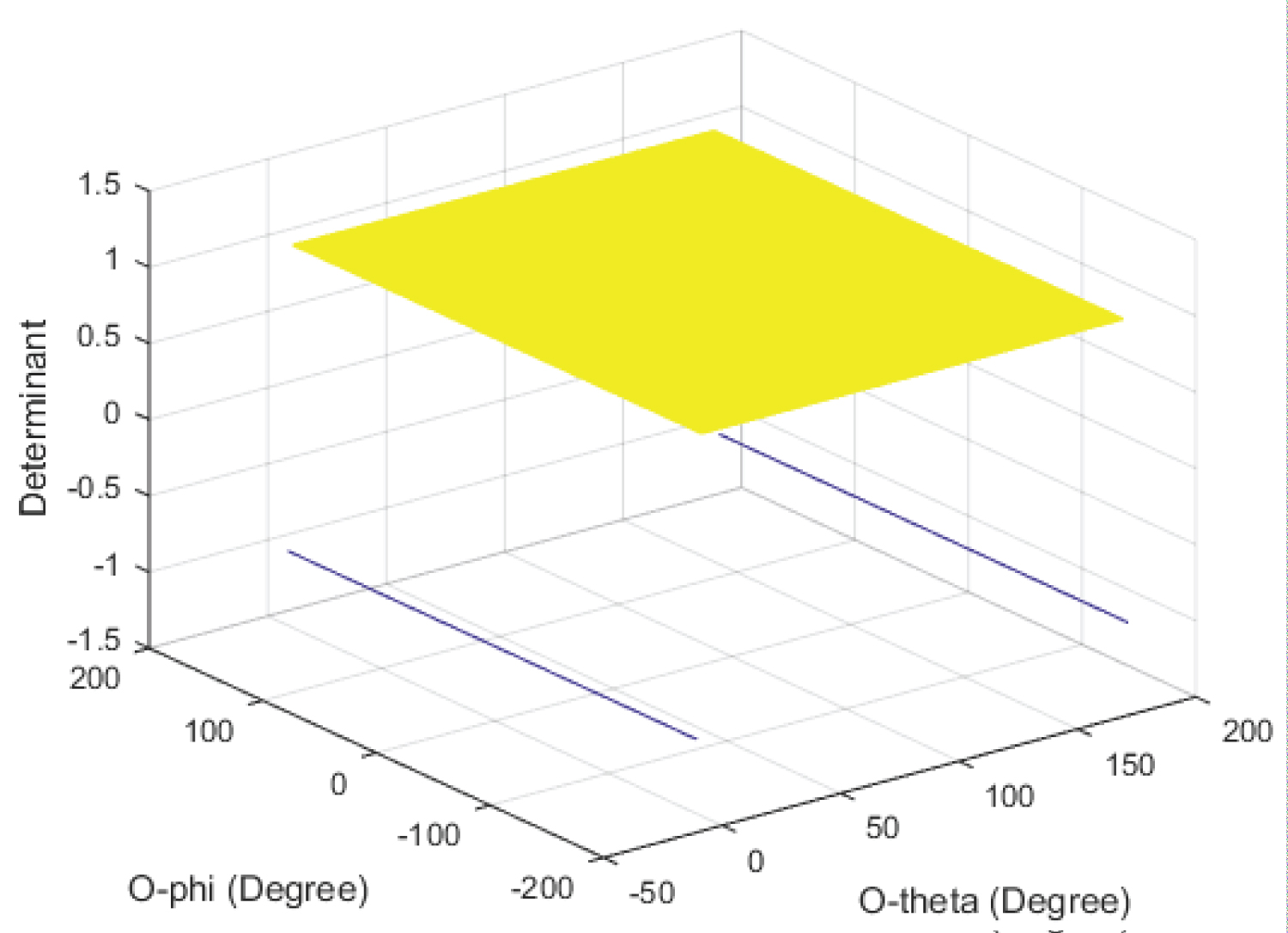
4) Plotting Determinant (7) with OΦ and Oθ using MATLAB:

Figure 12 shows the Determinant as a function in OΦ and Oθ Where OΦ varies from -180° to +180°, and Oθ from -1° to +181°.

5) Finding the limits at the borders of the surface:

The determinant points that need to be examined are at Oθ = 0° and Oθ = +180°.

Hooke's joint

1) Forward and Inverse Kinematics Equations:

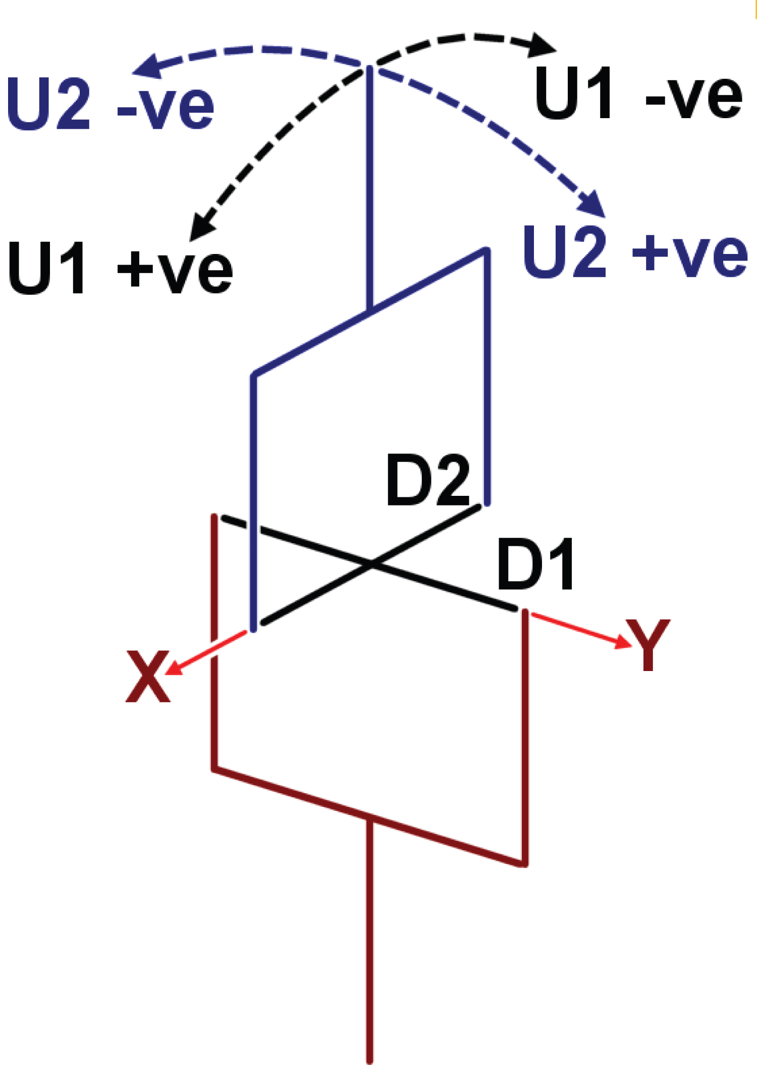
Figure 13 shows the joint-space variables of the Hooke's joint; U1 and U2 for both degrees of freedom D1 and D2, it also shows their positive and negative direction with respect to the X-axis and Y-axis:

Equation (8) shows the forward kinematics [17];

$$\left\{\begin{array}{l}\theta ={\cos }^{-1}\left(\cos \left(U2\right).\cos \left(U1\right)\right)\\ \Phi ={\tan }^{-1}\left(\frac{\left(\sin \left(U2\right)\right)}{\left(\cos \left(U2\right).\sin \left(U1\right)\right)}\right)\end{array}\right\}\left(8\right)$$

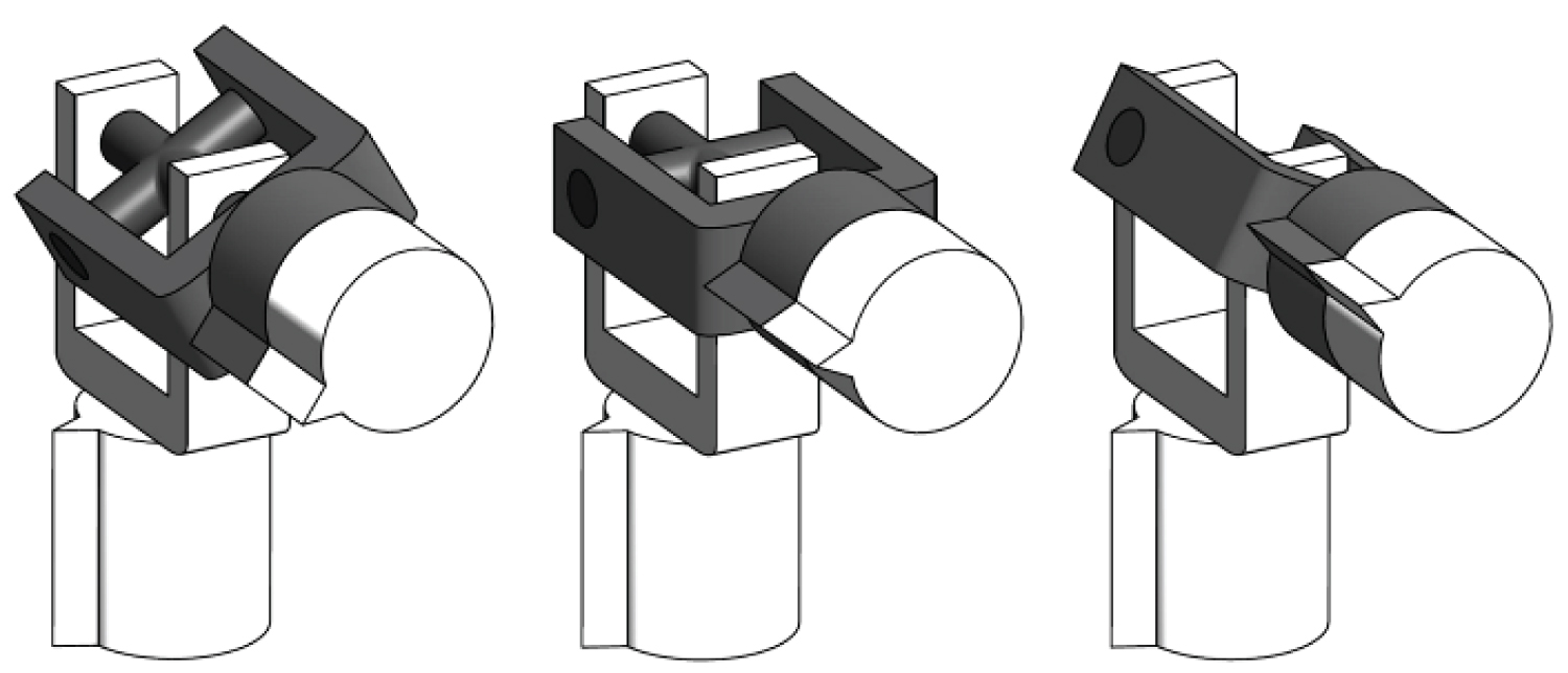
When the U2 = ±90°, U1 becomes irrelevant. However, It can only vary within this range [-90°,90°] due to physical limitations. At any of these two postures, the Hooke's joint has infinite solutions as shown in Figure 14.

Some examples:

Case a) For U1 = 0°, U2 = 90°, Substituting in (8);

θ = 90°, Φ = 90°.

Case b) For U1 = 30°, U2 = 90°, Substituting in (8);

θ = 90°, Φ = 90°.

Case c) For Oθ = 60°, U2 = -90°, Substituting in (8);

θ = 90°, Φ = -90°.

Case d) For Oθ = -70°, U2 = -90°, Substituting in (8);

θ = 90°, Φ = -90°.

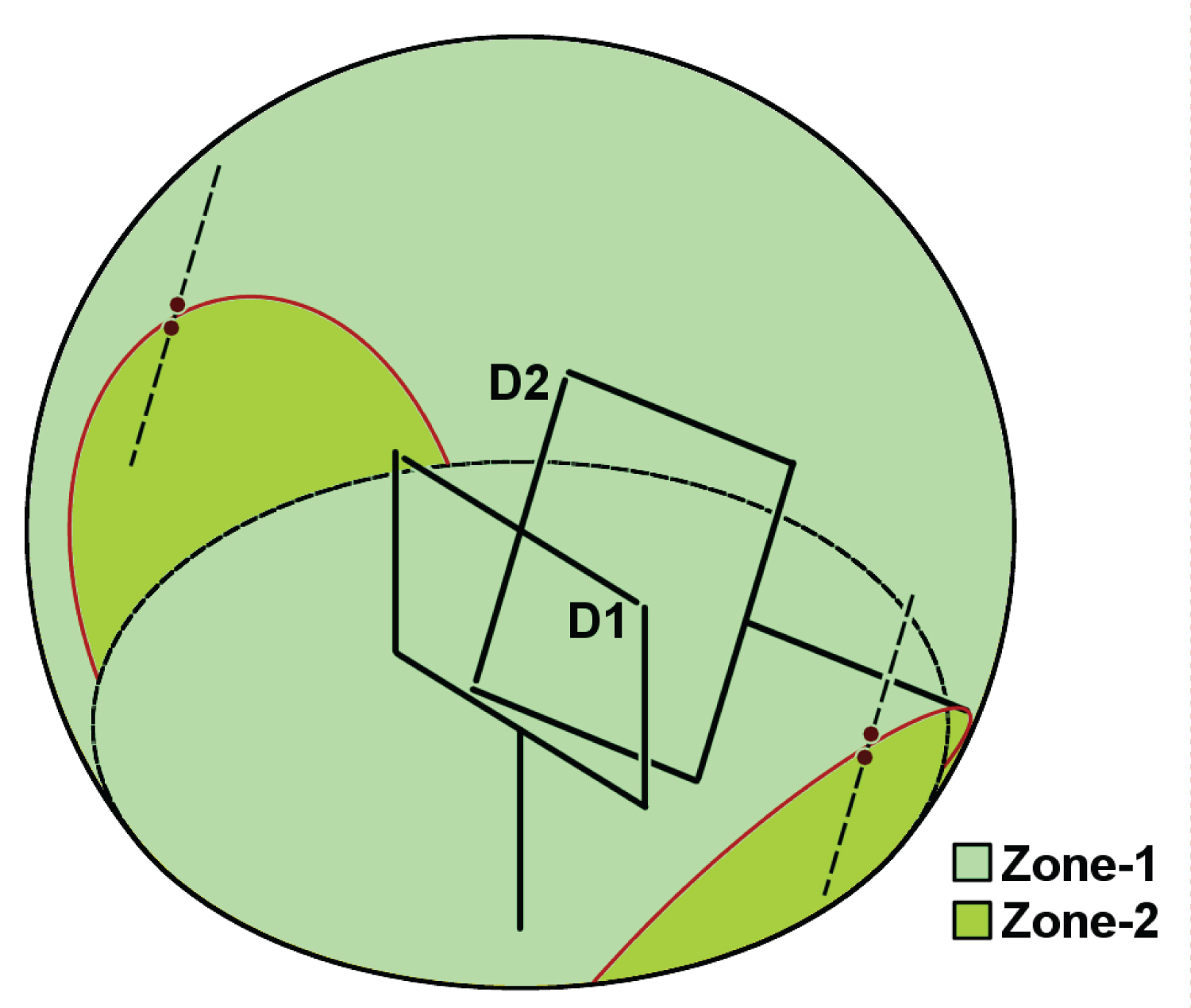
Figure 15 shows the range of field of motion for the Hooke's joint, with a deviation angle of 120°. The field of movement is divided into two zones Zone-1 and Zone-2. This is due to the fact that the joint will self-obstruct itself at certain postures:

Equation (9) [17] shows the inverse kinematics of the Hooke's joint and which zone and solution to pick according to U1 and U2, it also shows the points with infinite solutions:

$$\left\{\begin{array}{l}U1={\tan }^{-1}\left(\frac{\left(\sin \left(\theta \right),\cos \left(\Phi \right)\right)}{\left(\cos \left(\theta \right)\right)}\right),U2={\tan }^{-1}\left(\frac{\left(\sin \left(\theta \right).\sin \left(\Phi \right)\right)}{\left(\sqrt{{\sin }^2\left(\theta \right).{\cos }^2\left(\Phi \right)}+{\cos }^2\left(\theta \right)\right)}\right)\\ zone\_1,\left|U2\right|<{180}^o-\left|U1\right|\\ U1={\tan }^{-1}\left(\frac{\left(-\sin \left(\theta \right).\cos \left(\Phi \right)\right)}{\left(-\cos \left(\theta \right)\right)}\right),U2={\tan }^{-1}\left(\frac{\left(\sin \left(\theta \right).\sin \left(\Phi \right)\right)}{\sqrt[-]{{\sin }^2\left(\theta \right).{\cos }^2\left(\Phi \right)+{\cos }^2\left(\theta \right)}}\right)\\ zone\_2,\left|U2\right|>{180}^o-\left|U1\right|fromthe1stsetofsolution\\ U1\in ]-{90}^o,{90}^o[,U2=\sin \left(\Phi \right),{90}^o;\\ \Phi =\pm {90}^o+h{.180}^o,\theta =\pm {1.180}^o,handiare\mathrm{int}egers.\end{array}\right\}\left[9\right]$$

Actually the first two expressions are enough to find the values of U1 and U2. The last expression is only useful that it limits the value of U1 between -90 and 90 due to physical limitations, instead of it being undefined to have any value.

$$\left[{}_{\stackrel{.}{\varphi }}^{\stackrel{.}{\theta }}\right]=J\left[{}_{\stackrel{.}{U2}}^{\stackrel{.}{U1}}\right]$$

$$J=\left[\begin{array}{l}\frac{\partial \theta }{\partial U1}\frac{\partial \theta }{\partial U2}\\ \frac{\partial \varphi }{\partial U1}\frac{\partial \varphi }{\partial U2}\end{array}\right]$$

Using MATLAB;

$$J=\left[\begin{array}{l}\frac{\cos \left(U_2\right).\sin \left(U_1\right)}{\sqrt{1-{\cos }^2\left(U1\right).{\cos }^2\left(U2\right)}}\frac{\cos \left(U1\right).\sin \left(U2\right)}{\sqrt{1-{\cos }^2\left(U1\right).{\cos }^2\left(U2\right)}}\\ \frac{\partial \varphi }{\partial U1}\frac{\partial \varphi }{\partial U2}\end{array}\right]$$

3) Derivation of the Determinant with respect to U1 & U2.

Using MATLAB; the determinant is derived, and it is a long expression with real and imaginary parts. However it is plotted directly.

4) Derivation of the Determinant with respect to θ&φ:

Substituting (7) in (8) to get the Determinant with respect to θ and φ. While taking into consideration that there will be two equations, one for Zone-1 and one for Zone-2. Using MATLAB; the determinant is derived, and it is a long expression with real and imaginary parts. However it is plotted directly.

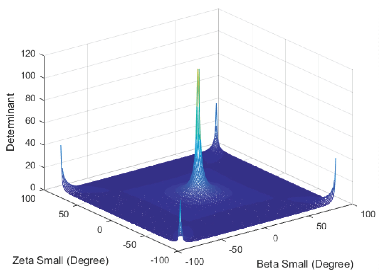
5) Plotting Determinant with U1 and U2 using MATLAB:

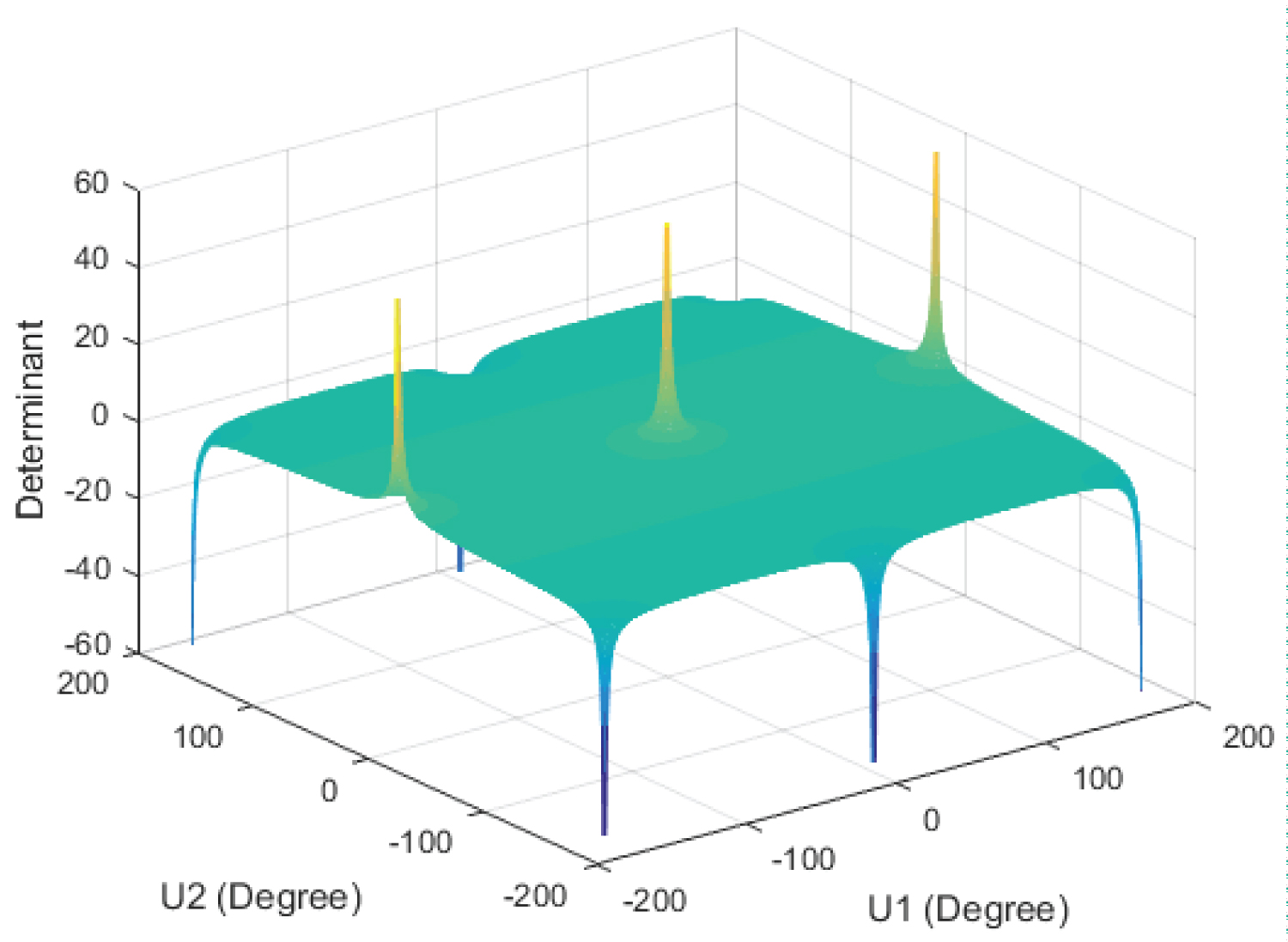
Figure 16 shows the Determinant as a function in U1 and U2 Where U1 varies from -180° to +180°, and U2 from -180° to +180°.

6) Finding the zero values of the Determinant:

The determinant points that need to be examined are at U2 = ±90°.

7) Plotting Determinant with θ & φ using MATLAB:

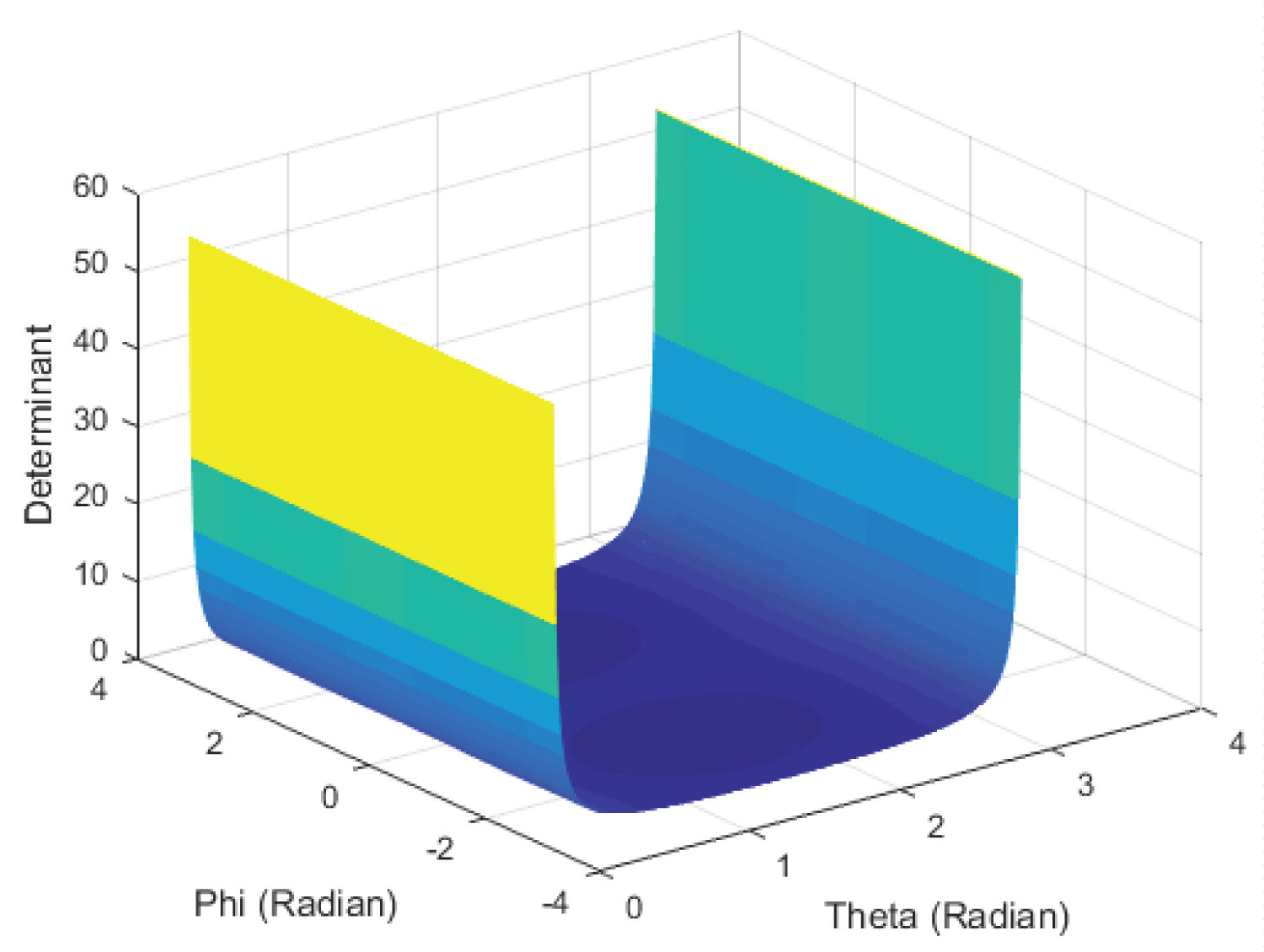
Figure 17 shows the Determinant of the solution from Zone-1 as a function in θ&φ: Where θ varies from 0° to +90°, and φ from -180° to +180°.

8) Finding the zero values of the Determinant:

The Determinant points that need to be examined are at θ = 90° and ϕ = ±90°.

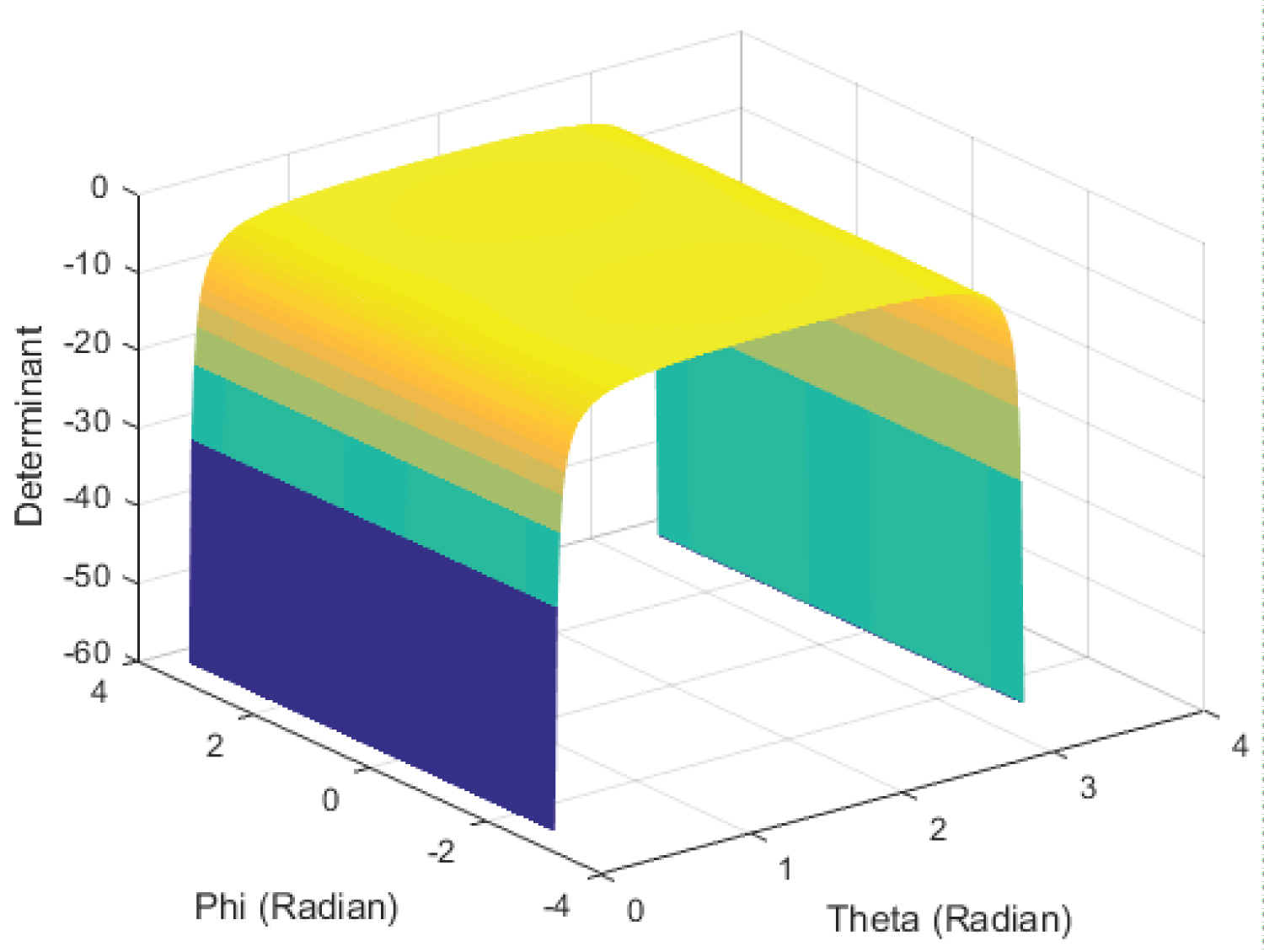
9) Plotting Determinant with θ&φ using MATLAB:

Figure 18 shows the Determinant of solution from Zone-2 as a function in θ&φ: Where θ varies from 0° to +90°, and φ from -180° to +180°.

10) Finding the zero values of the Determinant:

The determinant points that need to be examined are at θ = 90° and ϕ = ±90°.

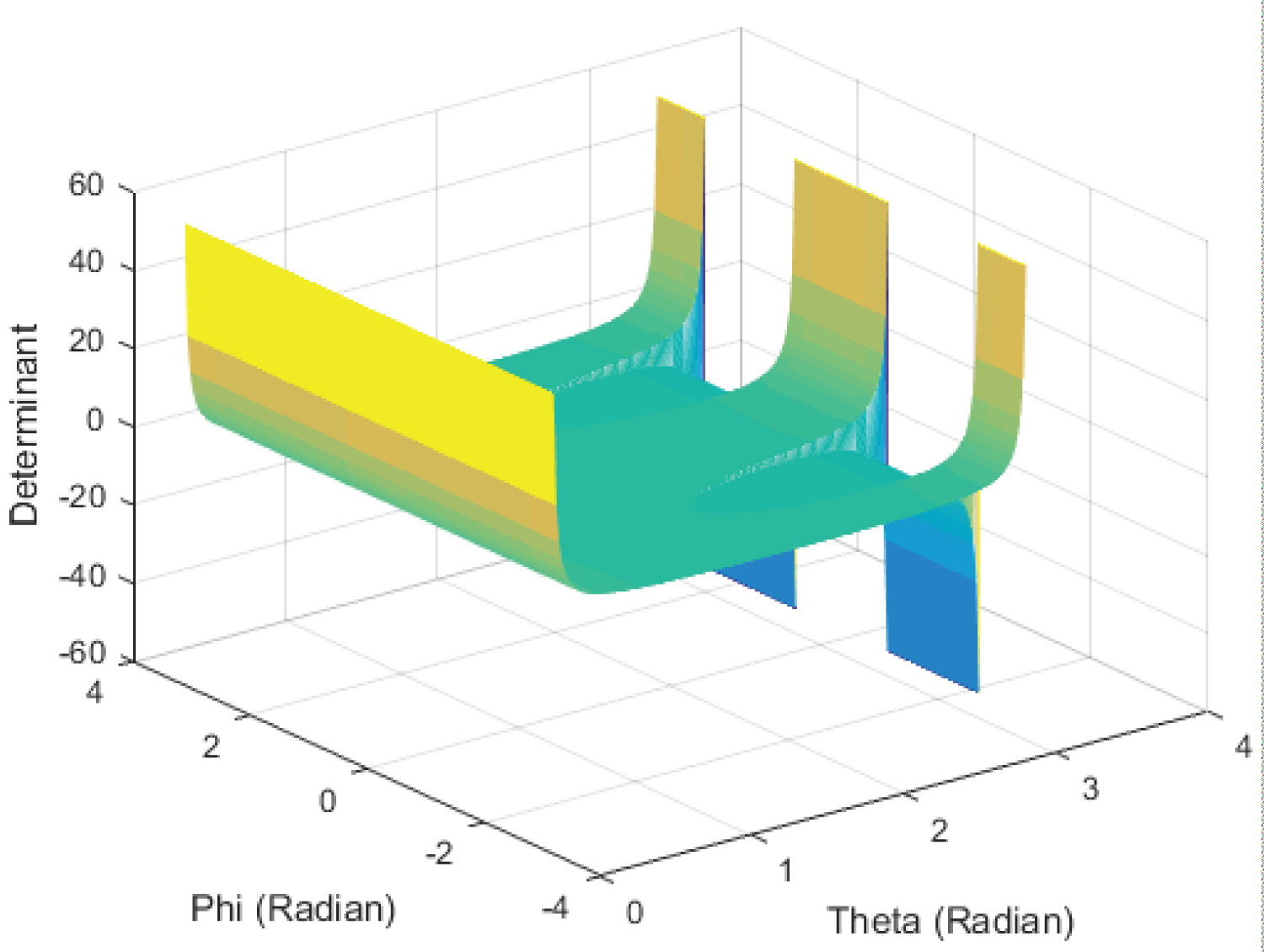
11) Plotting Determinant with θ&φ using MATLAB:

Figure 19 shows the determinant of solution according to Zone-1 or Zone-2 as a function in θ&φ: Where θ varies from 0° to +90°, and φ from -180° to +180°.

12) Finding the zero values of the Determinant:

The determinant points that need to be examined are at θ = 90° and ϕ = ±90°.

Results

For the Omni-Joint; the determinant as plotted in Figure 20 is not equal to zero on the entire surface, except at the borders it is undefined. The limits at the points on the borders approach zero. The determinant as plotted in Figure 21 is equal to zero at the border where θ = 180° [just past the spikes]. These results were checked using MATLAB.

For the Ordinary-Joint; the determinant as plotted in Figure 12 is equal to one on the entire surface, except at the borders (where Oθ = 0° and Oθ = +180°) it is undefined. The limits at the points on the borders are also undefined. However the value of the Determinate is equal to -1 just past the borders (at Oθ = -1° and Oθ = +181°). These results were checked using MATLAB.

For the Hooke's Joint; the determinant as plotted in Figure 16 is only equal to zero at U2 = ±90°, which is equivalent to θ = 90° and ϕ = ±90°. These results were checked using MATLAB.

Conclusions and Discussion

For the Omni-Joint; even though that the values at the borders of the surface shown in Figure 20 are undefined, the limits of these points are equal to zero. Which indicates that the Omni-Joint has a singularity when θ = 180°. Figure 21 confirms this, as the value of the determinant at θ = 180° is equal to zero. In addition (1) and (2) show that the Omni-Joint has one-to-one mapping as long as the deviation angle θ of is not equal to 180°.

For the Ordinary joint, Figure 12 showed that the Determinate is undefined at Oθ = 0° and Oθ = 180°, which may confirm that the Ordinary joint has singularities at these points, such as a physical prototype examination would proof. In addition (6) shows that the Ordinary joint is not one-to-one mapping.

For the Hooke's Joint, Figure 16 showed that the Determinate is equal to zero at U2 = ±90°. In addition Figure 17, Figure 18, and Figure 19 show that the Determinate is equal to zero at θ = 90° andφ = ±90°. These confirm that the Hooke's joint has singularities at these points. In addition (8) and (9) show that the Hooke's joint is has one-to-one mapping with discontinues range of field of motion.

These data show that that:

The Omni-Joint is singular free, except when the deviation angle is equal to 180°. And has the advantage of having one-to-one mapping, except when the deviation angle is equal to 180°.

The Ordinary joint suffers from two singularities when the deviation angel is equal to 0° or 180°. It is not one-to-one mapping.

The Hooke's joint suffer from two singularities when the deviation angle is 90° at an azimuth angle equal to ±90°, other that these two postures it has one-to-one mapping. However its range of field of motion is discontinuous.

References

1. Shah P, Patil AV (2016) Modelling & FEA of Universal Coupling of an Automobile Truck. International Journal for Innovative Research in Science & Technology 3: 391-402.
2. Williams RL (1999) Inverse Kinematics and Singularities of Manuipulatorswith Offset Wrist International Journal of Robotics and Automation 14: 1-8.
3. Williams RL II. June (1999) Singularities of a Manipulator with Offset Wrist. Journal of Mechanical Design 121: 315-319.
4. Arora R (2017) Modeling and Failure Analysis of Universal Joint using ANSYS”. International Journal of Emerging Technologies in Engineering Research 5.
5. Jawale HP, Thorat HT (2012) Investigation of Positional Error in Two Degree of Freedom Mechanism With Joint Clearance. J Mechanisms Robotics 4: 011002.
6. Han H, Park J (2013) Robot Control near Singularity and Joint Limit Using a Continuous Task Transition Algorithm. International Journal of Advanced Robotic Systems.
7. Binbin P, Zengming L, Kai W (2011) Kinematic Characteristics of 3-UPU Parallel Manipulator in Singularity and Its Application. International Journal of Advanced Robotic Systems.
8. Garcia-Sillas D, Gorrostieta-Hurtado E, Vargas JE, et al. (2015) Kinematics modeling and simulation of an autonomous omni-directional mobile robot”. Ingenieríae Investigation, 35: 74-79.
9. Djebrani S, Benali A, Abdessemed F (2011) Modelling and feedback control of an omni-directional mobile manipulator.IEEE International Conference on Automation Science and Engineering.
10. Xie Y, Yu J, Zhao H (2018) Deterministic Design for a Compliant Parallel Universal Joint With Constant Rotational Stiffnes. J. Mechanisms Robotics 10: 031006.
11. Cheng G, Wang S-t, Yang D-h, et al. (2015) Finite Element Method for Kinematic Analysis of Parallel Hip Joint Manipulator. J Mechanisms Robotics 7: 041010.
12. Pan H, Chen G, Kang Y, et al. (2021) Design and kinematic analysis of a flexible-link parallel mechanism with a spatially quasi-translational End Effector J. Mechanisms Robotics 13: 011022.
13. Lin S, Wang H, Zhang Y, et al. (2020) Kinematic geometry description of a line with four positions and its application in dimension synthesis of spatial linkage. J. Mechanisms Robotics 12: 031006.
14. Duta, Opera, Stanisic MM (1989) Dextrous Spherical Robot Wrist”. Patent US 4,878,393.
15. Zaied A, Ezzat AA, El Saeid, et al. (2007) New Robotic Joint Configuration.
16. Zaied A, Ezzat AA, El Saeid, et al. (2010) Joint. Patent PCT/EG2010/000037. Print.
17. Zaied A, Ezzat AA (2019) Omni-Joint: Proof of Concept, & Comparative Study. The American University in Cairo, DAR (Digital Archive and Research Repository of The American University in Cairo).