Real Application for a Low-Cost Low-Power Self-Driving 1/10 Scale Car

Abstract

In this paper, we discuss a real-life application for a low-power and low-cost self-driving car on a 1/10 scale platform. We present algorithms developed to achieve driving autonomy on a Low Power Single Board Computer using an ARM-based processor in a controlled environment. The authors provide insight on the usability of this technology for gait and performance running analyses. We perform walking and running analyses on an indoor athletic track over an autonomous follow-cam configuration. Through testing, we demonstrate how the vehicle can produce reliable and clinically valuable data. We discuss possible improvements and present recommendations for future works.

Keywords

Computer vision, Single board computer, Self-driving, Locomotion analysis, Low power computer, Autonomous driving, Raspberry Pi 4

Introduction

In early 2019, Tesla's CEO, Elon Musk, presented the company's first computer and chip to the world, named Full Self-Driving or FSD, capable of processing up to 2.5 billion pixels per second [1], an astonishing engineering feat. Although very impressive, many researchers and labs cannot afford or access this kind of computing power on portable devices for self-driving development. However, there are now many available options on the market capable of decent computing power at the lower end of the price range. For instance, let us think of the popular Nvidia Jetson Nano embedded computer or the even more popular, less brain-powered option, the Raspberry Pi 3B+. Though capable of self-driving on paper, very few studies present models with real-life conditions [2], reliability, scalability or specific applications other than following lane markings within closed lab doors [3,4].

This paper presents the full development of a 1/10 scale car equipped with a Raspberry Pi 4 capable of what would be considered as level 3 autonomous driving [5] used for the clinical analysis of locomotion.

Objective

The basis of this research is to perform quantitative motion analysis such as running and walking [6] through a moving visual referential based on the subject's position. An indoor athletic track and field was selected as a control environment. The research takes place at a University featuring an atypical 168-meter 4-lane indoor track. Each lane has a common width of 1 meter with 5 cm white lane line markings. The single radius geometry conforms to the standards where the straight segment is twice the length of the inner radius, more precisely, a 16-meterspan in this case.

The secondary objective was to develop such an instrument using only low-cost devices capable of performing onboard computation, thus reducing the need for extra material. The limiting cost factor is of interest to compete with the currently used evaluation methods that are both affordable and well-established (ex. Paper-based checklist or timed evaluation using a stopwatch) [7,8]. Also, the system is developed to alleviate the use of wearable devices for conducting the gait analysis since such systems are often hard to use for a layperson in ecological settings [9].

Project Configuration

Mechanical components

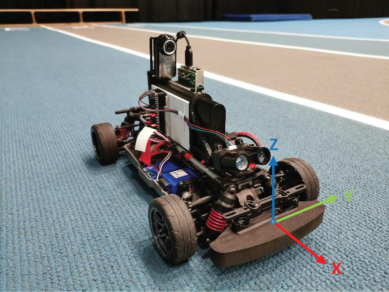
The robot structure is based on recommendations stated by the F1TENTH community [3]. It is built around the TRAXXAS 1/10 4-Tec 2.0 AWD Chassis (McKinney, Texas, United States) (Figure 1). This R/C dedicated scale chassis can reach speeds of up to 48 km/h (30 mph) and figures, as stated by its name, a four-wheel drive configuration with differential on both the front and rear of the car. The vehicle is equipped with two ¼ inch (6 mm) steel rods functioning as mounts for the electronics. The assembly is mainly achieved with various 3D printed brackets and supports.

Electronic components

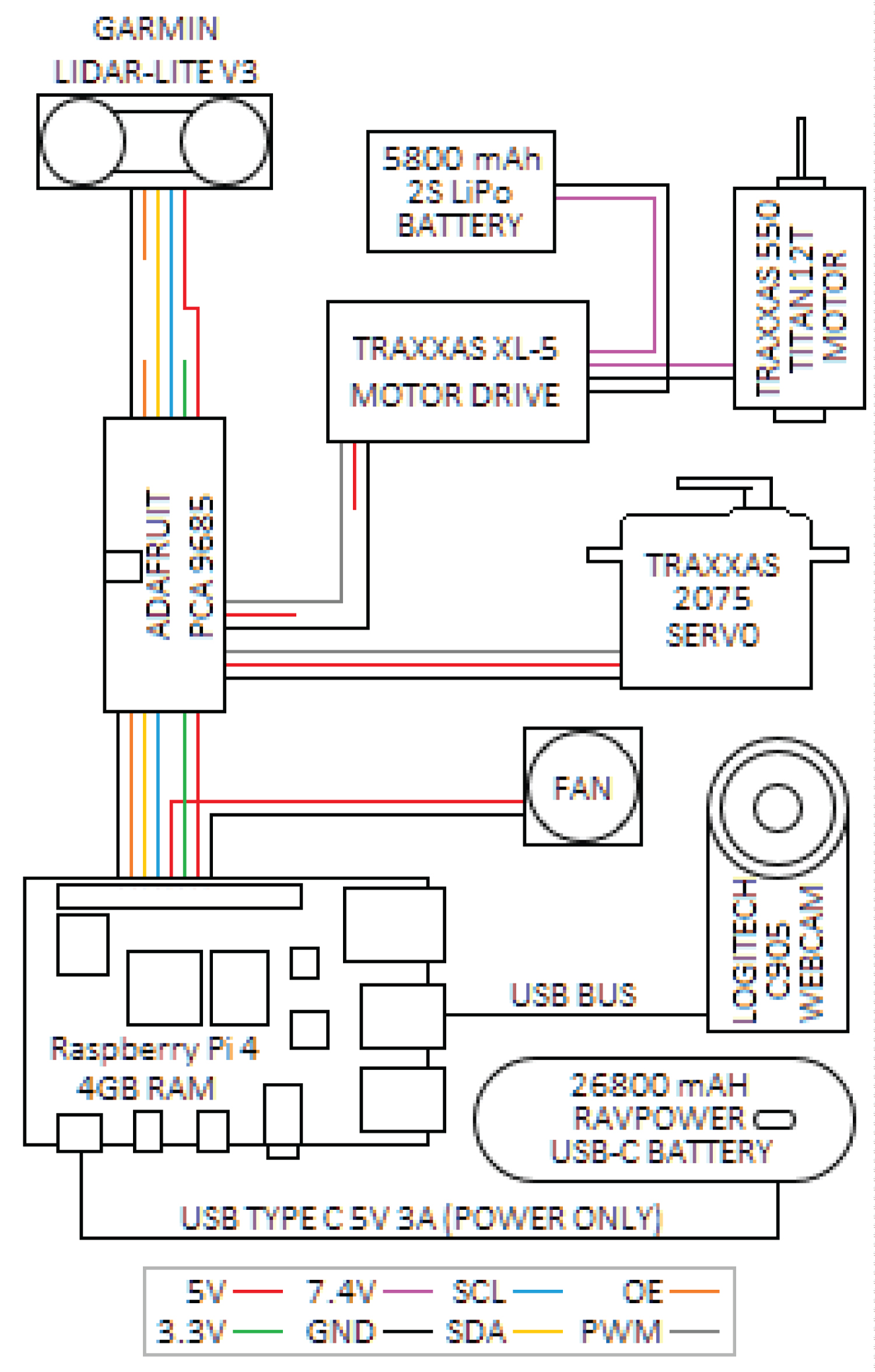
The computer module selected is the Raspberry Pi 4 (RP4) with 4GB of RAM (Cambridge, England). It has been equipped with a 32 GB Kingston Class 10 micro SD card (Fountain Valley, California, United States) for storage. The car comes stock with a TRAXXAS XL-5 Electronic Speed Controller (ESC), a Titan 12T brushed DC motor and a robust 2075 Waterproof servomotor. Both apparatus, the servomotor and the ESC, can be controlled via pulse modulation width (PWM). Though capable of producing software PWM throughout its general-purpose inputs and outputs (GPIO), the signal is too noisy to generate precise inputs for the ESC and the steering servomotor. To overcome this issue, an Adafruit PCA-9685 PWM (New-York, New-York, United States) driver board was added to the vehicle assembly. This device allows the RP4 to generate precise PWM via an I²C protocol and can be powered directly the computer. To conduct reliable subject following experiments, the robot was implemented with the Garmin LiDAR-LITE V3 (Olathe, Kansas, United States), a high precision laser distance sensor compatible with the RP4 I²C protocol. Lastly, the system uses a Logitech c905 (Lausanne, Switzerland) webcam as an RGB input directly connected to the RP4 USB port. Figure 2 shows the wiring diagram of the final assembly.

Power

With simplicity in mind, robot assembly has been rigged with two independent power sources. A 7.4 V 5800 mAh 2s battery pack from the car manufacturer was used for propulsion, whereas a RAVPower 5 V 26 800 mAh USB type-C power bank was used to power the main computer and peripheral devices. This decision was also made to avoid the need of a voltage converter and to extend the robot's battery life.

Software and project requirements

The RP4 runs on Raspbian, now called Raspberry Pi OS, a Debian-based operating system optimized for the Raspberry Pi product line.

Table 1 lists the libraries and the version used.

The entire code for this project was written in Python3, version 3.7.4. Many open-source libraries were needed to achieve this level of driving autonomy. Apart from the libraries needed for the integration of the sensor suite, Opencv, numpy and scipy were mainly used to complete this project.

Project architecture

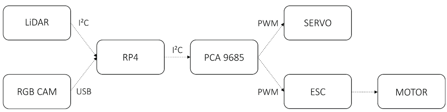
The project follows a rather simple architecture to reduce calculations and computing time. Information flows through the node sequentially without threads, as shown in Figure 3. Communication protocols are identified and represented by dashed lines. The robot performs its tasks by first reading the RGBcamera input and generating an output value through a controller. It then acquires data from de LiDAR sensor, providing the necessary values to perform a throttle output evaluation through another distinct controller. Values are then transferred to the PCA 9685 module by the RP4 via the I²C protocol which then outputs the signals to the ESC and to the steering servomotor, thus inducing trajectory modifications on the vehicle. The loop is repeated as long as needed, but can be stopped at any time by the evaluator or if the algorithm raises any safety concerns.

Computer Vision and Control Systems

Lane line detection

One of the key elements of the complete project is the use of a Low Power computer to perform a self-driving task. Though powerful enough to perform small artificial intelligence tasks, the RP4 is not optimized for neural network computations or machine learning training, which lead to the decision to produce a computer vision algorithm instead. As a matter of fact, the analysis environment of the project is sufficiently well-known and standardized to not require a more general approach line of a convolutional neural network. Many open-source lane detection algorithms are already available from a vast selection of suppliers, but none seemed to fit the needs of the project. Most of the codes available offer self-driving abilities with restricted capabilities. Projects often tend to use non-standard markings and scaled lane widths while not offering the speed capabilities anticipated by the team. To overcome these issues, it was decided that a computer vision algorithm would be developed, thus enabling self-driving in real-life conditions and applications, in our case within athletic track markings. Most of codes available over the Internet regarding lane detection tend to use the Canny edge detection over an area of interest (lane marking areas, generally the lower part of the input image) and then identify linear patterns with the Hough transform algorithm [10]. These patterns are returned as line extremums, then sorted as left and right line components and finally added to the evaluated frame for visualization. Though visually pleasing, this method does not provide a good approximation for curved lines, nor a mathematically valuable tool for trajectory evaluation.

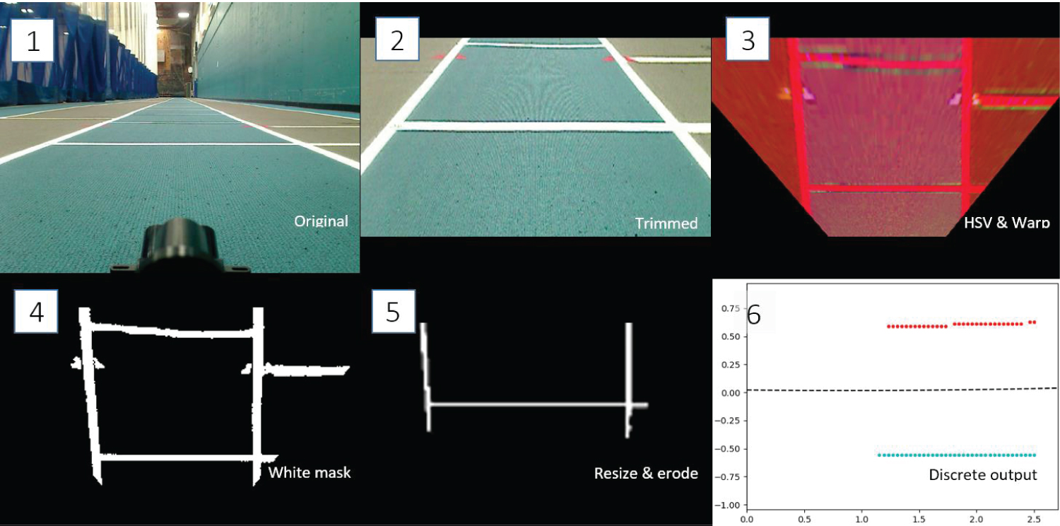
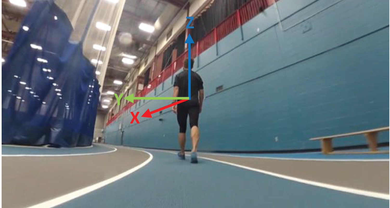
The lane detection code written for this project is in part based on the Ross Kippenbrock algorithm [11]. An RGB 960 × 170 resolution camera image is first fed into the program trimmed to remove over horizon area and resize to a 300 × 170 size to lower computational costs. The image is then modified via a warp function to create a synthetic bird's eye view. Using a color mask function, the lane linepixels are then selected according to their color and shade. An eroding function is applied to filter noise, thus removing undesired pixel agglomerates. To extract a discrete output from a pixel array, the image is then resized to about fifty percent of its original size. Selecting only the brightest pixels (closest to [255, 255, 255]), an array of around 200 points is created from the original image. Points are then rotated according to the vehicle coordinates (forward corresponding to +x axis and left +y axis as seen in Figure 1). The origin is at the center of the vehicle. To achieve reliable line sorting, we developed a robust algorithm. A vertical pixel sum of the first half of the resulting image is performed, generating a pseudo signal according to the predominance of white pixels. Since the distance between the two lines is constant throughout the track length, we can perform a signal analysis on the sum array using the scipy.signal library. By considering the lane width as the predicted wavelength, a parameter of the library's find_peaks function, we can identify apex cause by the line markings. If more than two vertex were detected, we compare these values to previous results to avoid false line detection and select the two best options. By using the peaks as starting points for each line, we can define the slope angle of the segment formed by our initial point to the closest one. If this point is within a threshold, in the case of this study being 15, the next point is considered as being part of the line and added to a list. This threshold is derived from the maximum possible lane deviation (in degrees) of the innermost line of the track described as part of this research at a 2.5-meter distance (camera horizon) with an added error value of 5 degrees. The algorithm is repeated for each point, based on the last point added in the list and the previous slope angle as well as for each peak selected. This algorithm helps to remove perpendicular values and "off the chart" data. The code algorithm is presented below. Two 2nd degree polynomial equations representing lane lines are computed from the two separate data sets created. These two functions are then averaged to evaluate the estimated lane center.

Algorithm 1: Line data sorting.

lines_point[]

for points in position[] do

sort (x_i,y_i) where x_i < x_i+1 $\forall$ i

end for

histogram[] ← ${\Sigma }_{i=0}^{\raisebox{1ex}{$n$}\!\left/ \!\raisebox{-1ex}{$2$}\right.}$ image [i], n = image width for each rows in image height

peaks[] ← find_peaks(histogram[], track_widht)

peaks[] ←two best peaks compared to previous peaks[]

for peak in peaks[] do

last_theta ← 0

lst[] ← peak

for point in the point list[] do

theta ← angle between point and lst [-1]-last_theta

if theta < 15 then

lst.append(point)

last_theat ← theta+last_theta

end if

end for

lines_point.append(lst)

end for

Steering control

As shown in Figure 4, the computer vision algorithm produces a smooth and reliable ideal trajectory for the car to use as a goal. This 2^nd degree polynomial equation can be used to approximate the car's actual cross track error (CTE) by evaluating the function's value at the vertical intercept, the car being conveniently placed at the origin. The evaluated CTE is fed into a proportional-integral-derivative (PID) controller which then outputs a pulse width value converted into torque change by the motor. The robot was initially implemented with a simple model predictive control (MPC) using an in-house-developed mathematical steering model considering the four-wheel drive nature of the car. However, this method proved to be too time-consuming in terms of computing and was dropped early in the project.

Throttle control

While steering control is always performed according to lane line markings, the robot can carry out different assessments requiring a wide range of speed control patterns. Training and evaluation with predefined velocities, only required a user speed profile input. However, many analyses are based on the subject's speed. To achieve a constant distance with the subject, the vehicle utilizes an optical distance measurement sensor. Control of speed and distance is achieved through a PID controller, using the current subject/robot distance as an input and computing a throttling output for the ESC. As of right now, the PID parameters have been tuned using the Ziegler-Nichols method [12].

Data collection

The main goal of this research is to produce similar results as what would be possible for an in-lab visual locomotion analysis. Such evaluations are generally performed on a treadmill or over a controlled area and use a so-called global referential where the room is the spatial reference. In this project, using such a system would induce the need for real-time position estimation as well as complex computations to correctly evaluate the subject's locomotion patterns. As a bypass, it was decided that the spatial reference would be fixed to the subject, thus nulling the need for accurate position estimations, as shown in Figure 5.

Although many evaluation types can be performed using the robot, this paper will focus on a following evaluation (the robot is placed behind the subject being evaluated). The basics of this evaluation are simple. A distance or time is first selected by the evaluator to conduct the desired evaluation. A track lane must then be selected independently of its color or length to perform the evaluation, according to the test requirements. To ensure a good visual frame for image capture, the evaluator is encouraged to modify the goal distance between the subject and the vehicle. The set distance for this paper was 2.5 meters (≈100 inches). To engage an evaluation procedure, the vehicle is placed on the selected lane. Though the robot does not have to be perfectly placed in the center of the lane, positioning it on a fairly straight alignment and close to the middle will help the vehicle perform better from the beginning. The vehicle will recover the initial placement error within the first 5 meters. Critical positions include a plus/minus 45 cm away from the lane center and a plus/minus 30 degree offset from the lane center tangent. Once the car is placed as desired, the subject can take place in front of the vehicle. We recommend placing the subject somewhere between 50 to 25 percent closer to the set distance to avoid premature correction from the robot. The evaluator can then proceed with the car's program start-up. This can be achieved via the remote desktop application available on the Windows platform (Windows 10, Microsoft, USA). The robot's main computer has been programmed to generate a secure Wi-Fi network from which a remote computer can be connected to perform the assessment. A starting countdown will lead to the beginning of the test. The subject can then proceed with to walk and/or run.

Results

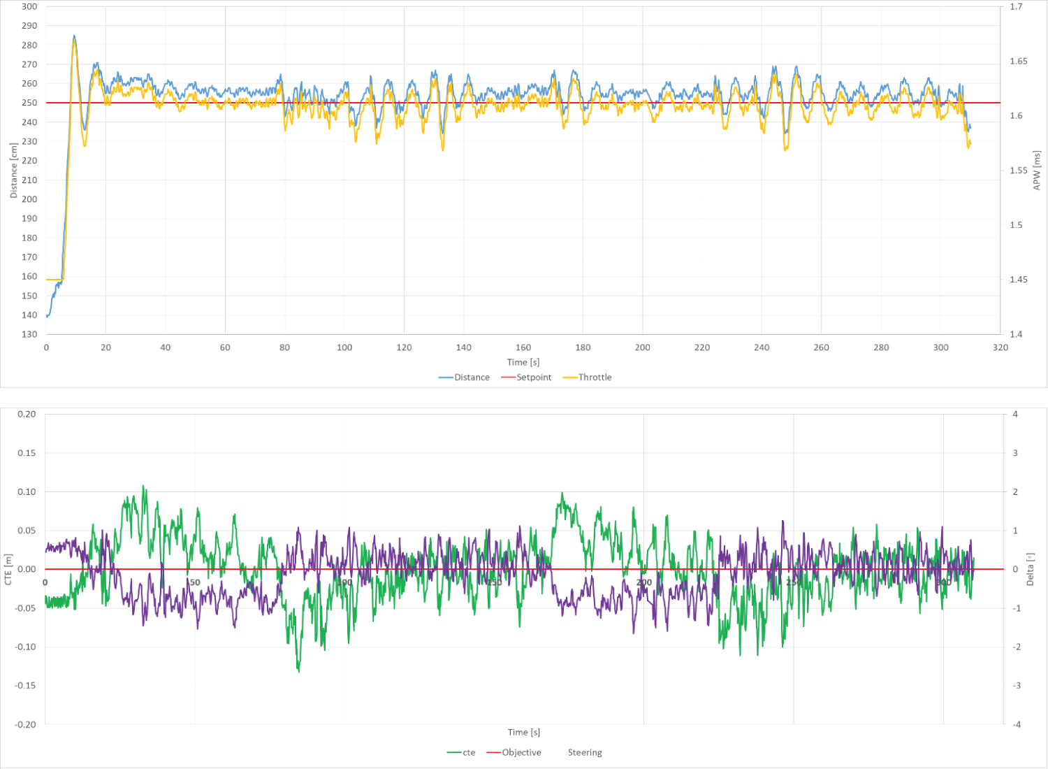
Trials were conducted through different testing which include a 180 m (600 ft.) walk (1.25m/s or 4.5km/h), a 180 m run (3.44 m/s or 12.4 km/h) and a trial at variable paces for 540 m (1800 ft.)(1.3, 1.5 and 2.5 m/s, or 4.7, 5.4 and 9 km/h, respectively). All tests were carried out on an indoor athletic track, as described in the objective. Experiments were conducted on two different subjects presenting no functional limitations or pathologies. Tests were conducted to better understand controller tuning and project limitations. Figure 6 presents the plotted results of the experiment, i.e. the CTE and steering output (δ) through time and the throttle output (APW) compared to the perceived distance (D) through time from the 555 m evaluation. All analyses were performed at an average rate of 10.1 Hz, a similar value to the 10.3 frames per second performed by the main computer when only the camera is in use with an external webcam app (Guvcviewer, http://guvcview.sourceforge.net/) at a 960 × 720 resolution.

Discussion

Overall, current results show that this platform is effective at providing quantitative data of gait parameters [6] using a self-driven vehicle in a quasi-controlled environment. Data show that further improvements are needed on the tuning of the PID values. As an example, even if gait induces a sinusoidal kinematic response, output extirpated from this analysis are too rough to represent it graphically. A 0.15 Hz frequency on the distance control can easily be observed in Figure 6a, a number too small to be expressed as a gait pattern [13]. Moreover, some analysis segments, as seen at 100 and 240 seconds, present more dramatic PID corrections over the period of 20 seconds with an amplitude variation of 20 centimeters. These variations could be explained by the subject's torso movements, which are currently considered as steady by the software.

Regarding the autonomous lane driving control, Figure 6 depicts adjustments made by the vehicle based on what is perceived and computed by the camera. A variability in the steering output can be observed, and is proportional to the input from the lane line detection, giving it a saw tooth appearance. We can observe that even small lane detection errors are also considered in the vehicle's direction. Further data filtering could help prevent steering overcompensation, thus providing the system with a smoother drive. A more restrictive line evaluation protocol could also be implemented to better discard "off the chart" line detection.

Such results are promising since we were able to perform basic motion analysis from a steady frame on a moving subject. Although further testing and tuning will be needed to demonstrate the robot's real capabilities, results obtained throughout this experiment demonstrate the feasibility of such tool.

Cost

The estimated cost of the required equipment for the current system is approximately $1,000CAD ($750). As presented by Müller & Koltun [2], this project is comparable to other low-cost vehicles developed for automated driving and racing. Moreover, the current system is a stand-alone platform for navigation in quasi-unrestrained environments since other systems are typically designed to track lines on a laboratory floor where the aim of the project is to "train" the system to go faster using machine learning or neural networks. Therefore, the developed system responds to our second objective which was to provide a low-cost device for the analysis of human movement.

Safety

Safety is a major concern when working with human and any living beings. To ensure the subject's safety throughout our testing, the robot was developed with some preprogrammed safety measures. A programmed safety switch was integrated to the code, making it possible to terminate any evaluation at any time from the remote computer, thus completely stopping the car. Another safety measure comes from the LiDAR coding. The code was implemented with a proximity warning that will ultimately stop the car and terminate the program if the robot comes too close to, or goes too far from a test subject or any other obstacle. Moreover, lane lines must be identified at all times to ensure that the car remains running. To overcome glitches and inaccuracies, the code can raise a maximum of 3 consecutive undetected line warnings before terminating, thus completely stopping the vehicle. If the wireless connection fails between the remote computer and the robot, the vehicle will also come to a complete stop.

Conclusion

The current work demonstrates that a low-cost low-power self-driving 1/10 scale car can be used to assess walking and running in a controlled environment. The data gathered is reliable and can be clinically valuable for health specialists when assessing one's mobility. Future studies will focus on implementing more complex analyses of human movement for the automatization and production of quantitative data to limb movements [14].

To produce more reliable analyses in the future, the vehicle could be equipped with a less restrictive distance-measuring device, such as a rotating LiDAR or even through visual estimations. More improvements on lane line detection should also provide the robot with a steadier control. The actual processing speed of 10 frames per second seems to be a limiting factor for the team in view of the maximum speed that can be safely reached by the robot. Further analysis and code modifications will be carried out to achieve a more efficient goal of 20 frames per second on the same hardware. Since the camera feed was identified as a limiting speed factor, a better, smarter, and faster U.S.B. 3.0 webcam could be implemented in parallel to a smaller input frame resolution.

Future work will include the onboard kinematic motion analysis to better understand human locomotion and further document motion patterns from this new perspective. Also, induced vibrations produced by the track deformities should be considered to better capture motion. Modern software can produce reliable video capture by numerical stabilization, which could be implemented in this project.

Acknowledgements

This work was supported by a grant from Centre intersectoriel en santé durable (CISD) of Université du Québec à Chicoutimi (UQAC).

References

1. Bos C (2019) Tesla's new HW3 self-driving computer-it's a beast (CleanTechnica Deep Dive). CleanTechnica.
2. Müller M, Koltun V (2020) OpenBot: Turning smartphones into robots. arXivLabs.
3. (2020) F1TENTH Foundation. F1TENTH.
4. Stranden JE (2019) Autonomous driving of a small-scale electric truck model with dynamic wireless charging. Norwegian University of Science and Technology.
5. Society of Automotive Engineers (2018) Taxonomy and definitions for terms related to driving automation systems for on-road motor vehicles. SAE International, 35.
6. Cimolin V, Galli M (2014) Summary measures for clinical gait analysis: A literature review. Gait and Posture 39: 1005-1010.
7. Owsley C, Sloane M, McGwin G, et al. (2002) Timed instrumental activities of daily living tasks: Relationship to cognitive function and everyday performance assessments in older adults. Gerontology 48: 254-265.
8. Wall JC, Bell C, Campbell S, et al. (2000) The timed get-up-and-go test revisited: Measurement of the component tasks. J Rehabil Res Dev 37: 109-113.
9. Stone EE, Skubic M (2011) Passive in-home measurement of stride-to-stride gait variability comparing vision and kinect sensing. Annu Int Conf IEEE Eng Med Biol Soc 2011: 6491-6494.
10. Canny J (1986) A computational approach to edge detection. IEEE Trans Pattern Anal Mach Intell 8: 679-698.
11. Keenan R, Kippenbrok R, Brucholtz B, et al. (2017) Advanced lane finding.
12. Ziegler JG, Nichols NB (1993) Optimum settings for automatic controllers. J Dyn Sys Meas Control 115: 220-222.
13. Winter DA (1993) Knowledge-base for diagnostic gait assessments. Med Prog Technol 19: 61-81.
14. Ramakrishnan T, Kim SH, Reed KB (2019) Human gait analysis metric for gait retraining. Appl Bionics Biomech 2019: 1286864.