Robust Adaptive Gaussian Mixture Sigma Point Particle Filter
Abstract
This paper presents a new robust adaptive Gaussian mixture sigma-point particle filter by adopting the concept of robust adaptive estimation to the Gaussian mixture sigma-point particle filter. This method approximates state mean and covariance via Sigma-point transformation combined with new available measurement information. It enables the estimations of state mean and covariance to be adjusted via the equivalent weight function and adaptive factor, thus restraining the disturbances of singular measurements and kinematic model noise. It can also obtain efficient predict prior and posterior density functions via Gaussian mixture approximation to improve the filtering accuracy for nonlinear and non-Gaussian systems. Simulation results and comparison analysis demonstrate the proposed method can effectively restrain the disturbances of abnormal measurements and kinematic model noise on state estimate, leading to improved estimation accuracy.
Keywords
Particle filter, Gaussian mixture sigma-point particle filter, Gaussian mixture approximation, Robust adaptive estimation
Introduction
The problem of nonlinear filtering has its origins in the areas of tracking and signal processing. However, the underlying setting is extremely general and is ubiquitous in many applied areas such as integrated navigation system, information fusion, signal processing, target tracking, fault detection, geodetic positioning and automatic control, where random processes are used to model complex dynamic phenomena. In essence, nonlinear filtering is to estimate the state of a nonlinear and non-Gaussian stochastic system from measurement data.
A significant amount of research efforts have been dedicated to nonlinear filtering. The extended Kalman filter (EKF), unscented Kalman filter (UKF) and particle filter (PF) are the typical nonlinear filtering methods. The EKF is an approximation method, in which nonlinear system equations are linearized by the Taylor expansion and the linear state is assumed to obey the Gaussian distribution. However, the linearization of system equations involve error, leading to biased or even divergent filtering solutions. Further, the EKF also requires the calculation of the Jacobian matrix, which is difficult to implement in practical applications [1,2]. The UKF overcomes the problems of the EKF by conducting nonlinear parameter estimation based on unscented transform. It can achieve third-order accuracy, while the EKF provides first-order accuracy only. However, the UKF performance is sensitive to system model error. Further, when the nonlinearity of a dynamic system is strong, the estimated state error will become large or even divergent.
The PF is an optimal recursive Bayesian filtering method based on Monte Carlo simulation by producing a sample of independent random variables according to a conditional probability distribution [3]. It is easy to implement, suitable for high-dimensional problems, and can deal with nonlinear and non-Gaussian models. However, the phenomenon of particle degeneracy may occur in the approximation process, and the accuracy heavily depends on the selection of the importance sampling density and resampling scheme [4-6]. Various methods were reported focusing on improvement of the importance sampling density and resampling scheme, such as the auxiliary PF, regularized PF and marginalized PF. However, these methods suffer from their own problems. The performance of the auxiliary PF will be degraded if the process noise is large. The particles generated by the regularized PF do not share a common distribution with the practical probability function, leading to the increased variance of state estimation. The marginalized PF is only suitable for the nonlinear system containing the linear state component [7,8].
Based on the Gaussian filter reported by Ito and Xiong [9], Van der Merwe, et al. proposed a Sigma-point particle filter (SPPF) and a Gaussian mixture Sigma-point particle filter (GMSPPF) for nonlinear systems [10,11], where the Sigma point is used to improve the importance sampling density. The Sigma point is a method to calculate the statistics of a random variable under a nonlinear transform. It makes use of unscented transform for the importance density and obtains third-order statistics for the estimations of state mean and variance. It can approximate posterior mean and covariance for a non-Gaussian and nonlinear system in the accuracy of at least second-order Taylor series. Therefore, both SPPF and GMSPPF have a better performance than the PF [9-11]. The SPPF requires the Gaussian approximations of each particle to conduct a system update, while the GMSPPF uses a multi-dimensional mixed ingredient for update of the entire particle set, leading to the superiority to the SPPF [12-14]. Further, as it moves particles to the high likelihood areas and subsequently uses a finite Gaussian to obtain the appropriate importance density function, thus the GMSPPF significantly reduces the computational load comparing to the PF and SPPF. However, the GMSPPF adopts the UKF to approximate the predicted prior and posterior density functions. If there are uncertainties involved in system and measurement noises, the UKF approximation would be deteriorated, leading to the biased solution of the GMSPPF.
Robust adaptive estimation utilizes the equivalent weight function and adaptive factor to control the information of the kinematic model and observation to inhibit the disturbances of systematic noises, leading to more accurate estimations of mean and covariance [15,16]. It can be combined with the PF by selecting an appropriate importance density function to handle the disturbances of system error on state estimation.
This paper presents a new robust adaptive Gaussian mixture sigma-point particle filter (RAGMSPPF) by introducing the equivalent weight matrix and adaptive factor into the UKF to improve the accuracy of Gaussian approximation and further enhance the GMSPPF performance. This method approximates state mean and covariance by Sigma-point transformation combined with the information obtained from new available measurements. Subsequently, it develops the equivalent weight function and adaptive factor to adjust the estimations of state mean and covariance to control the disturbances of singular measurements and kinematic model noise. Based on above, it obtains predicted prior and posterior density functions via Gaussian mixture approximation to improve the filtering accuracy for nonlinear and non-Gaussian systems. Simulations and comparison analysis have been conducted to comprehensively evaluate the performance of the proposed filtering method.
Gaussian Mixture Sigma Point Particle Filter
Consider the following nonlinear system
where is the state vector at epoch k, the system measurement at epoch k, the system state noise which is assumed to be a white noise with variance Qk, and the measurement noise which is assumed to be a white noise with variance Rk. Both f(·) and h(·) are a nonlinear function, and k = 0,1,… is the sampling time.
The basic idea of the Gaussian mixture sigma point particle filter (GMSPPF) is to use a finite Gaussian mixture model to construct the posterior density function, which is much closer to the actual density function [9-13]. In the time update, the predicted prior density is expressed as
and in the measurement update, the posterior density is expressed as
where and are calculated by constructing a parallel bank of UKFs [11]. αg represents the mixing weight, represents the Gaussian density function with mean vector and positive definite covariance matrix , and and where G, I and J are the numbers of mixing components in the state, process noise, and measurement noise, respectively.
Robust Adaptive Gaussian Mixture Sigma-Point Particle Filter
It can be seen from (2) and (3) that in the GMSPPF the predicted prior and posterior density functions and are approximated by the UKF. However, if there are uncertainties involved in system and measurement noises, the UKF approximation would be deteriorated, leading to the biased solution of the GMSPPF. This paper establishes a new RAGMSPPF by introducing the equivalent weight matrix and adaptive factor into the UKF to improve the accuracy of Gaussian approximation and further enhance the GMSPPF performance.
The RAGMSPPF algorithm can be described as the following steps:
Step 1: Initialization: at k = 0, define the initial prior probability density function in the form of N Gaussian mixtures, i.e.
where denotes the jth Gaussian weight, and
Step 2: The state mean and covariance are computed by the robust adaptive UKF algorithm.
(i) At epoch (k ≥ 1), calculate 2n + 1 Sigma points as
where is the scaling parameter, ax determines the spread of the Sigma points around and is usually set to a small positive value, and k is the secondary scaling parameter which is usually set to zero
Wi is the weight associated with the ith Sigma-point such that ƩWi = 1, i = 0,1,…2n. Wi (I = 0,1,…2n) are set as
where β is used to incorporate the prior knowledge on the distribution of x in the filtering process. For the Gaussian distribution, β = 2 is optimal.
(ii) Considering the current measurement, calculate the Gaussian approximation function , and further propagate the approximated mean, covariance and cross covariance via the Sigma-point transformation as follows
(iii) Calculate the equivalent weight matrix and the adaptive factor α [16-18]. The equivalent weight matrix is constructed using the IGG scheme [16] to incorporate the robustness constraint in measurement via a descending weight function. In case of independent variables, the equivalent weight matrix is a diagonal matrix with the diagonal element represented as
An alternative expression of is
where pk is the kth main diagonal element of the covariance matrix of the measurement vector zk; and ; and is the residual vector of zk.
To balance the contributions of the predicted state and measurement to the state estimation, the adaptive factor γk is represented as the following piecewise decreasing function
where and and , tr(·) represents the matrix trace, and and Pk denotes the state estimation and the corresponding covariance [17,18].
It can be seen from above that the equivalent weight and adaptive factor are in a similar form, and they both are the adjustment factors. The former is determined from the residual, while the latter is determined from the difference between the state estimation and state prediction, i.e., . Using the equivalent weight matrix and the adaptive factor, the estimate and variance can be obtained as follows
where
It can be seen from the above equations that can be adjusted via γk and , thus effectively controlling the utilization of kinematic model information and measurement information to restrain the disturbances of singular measurements and kinematic model noise.
Step 3: Calculate the posterior probability density function.
where Nf = NNn is the total number of mixing components in the measurement update, and Nn is the number of mixing components in the measurement noise. The jth posterior probability density can be obtained from (5)-(21), and the mixing weights are
where
Equation (22) can be viewed as the importance density function. It can be seen from (20) that can be adjusted via γ and , making the important density function described as (22) closely approximate the practical density function. It can be seen from (16), when there is singularity involved in the measurement model, the residual vector Vk will be enlarged, thus reducing the components of equivalent weight matrix and enlarging the predicted measurement covariance . Subsequently, it is readily known from (21) that the gain matrix will be reduced. As a result, as can be seen from (19) the use of measurement information in the estimation will be reduced, thus restraining the disturbance of singular measurement on the state estimation.
Similarly, the adaptive factor γk is reduced when there is noise involved in the kinematic model. Consequently, the utilization of state prediction information in state parameter estimation is reduced, inhibiting the disturbances of the kinematic model noise. If and γ = 0, then are the mean and covariance matrix obtained by the standard UKF.
Step 4: Similar to the calculation of the posterior probability density function, the predicted density function is approximated by
where Np = NfNv is the total number of mixing components in the time update, and Nv is the number of mixing components in the measurement noise. The jth predictive probability density can be obtained from (8), (9) and (14), and the mixing weights are represented by
where
Step 5: Calculate the particle weights.
Normalize the weights
Step 6: The PF resamples the particle in a new set of equally weighted particles, but the RAGMSPPF approximates the density function in a Gaussian form, that is, obtains mean and covariance in time series recursively. In order to avoid the massive number of particles due to resampling and reduce the particle degeneracy phenomenon and computational complexity, applying the weighted expectation-maximization technique [11] to fit the set of weighted particles with the posterior N-component Gaussian mixture model, we can readily have
Step 7: Repeat Steps 2 to 6 until all samples are processed.
Simulation Analysis and Discussions
Simulations were conducted to comprehensively evaluate and analyze the performance of the RAGMSPPF method. The comparison analysis with the PF and GMSPPF methods is also discussed in this section.
Lognormal probability density
For comparison, simulations were conducted under the same conditions by the proposed RAGMSPPF as well as the PF and GMSPPF, respectively. Consider the state and measurement models [19].
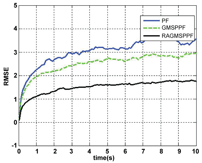
where Q = 1, and R = 1. The sampling time was Δt = 0.25s and measurements were updated every 0.1s. The particle number for the PF was set to 500. A 5-3-1 scheme (a 5-component GMM (Gaussian Mixture Model) for the state posterior, a 3-component GMM to approximate the process noise, and a 1-component GMM for the measurement noise) was used in the GMSPPF and RAGMSPPF. The estimation accuracy for the nonlinear system was calculated in terms of root mean square error (RMSE), which is defined as
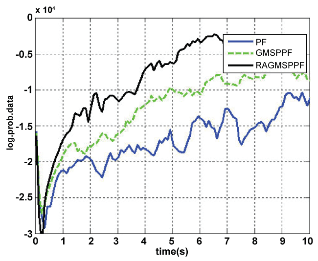
When the nonlinear system is of multi-dimensional distribution, the state estimations of the PF, GMSPPF and RAGMSPPF are compared in terms of the lognormal probability density defined by
where and are obtained from the above three filters, respectively. It can be seen from (32) that the larger the lognormal probability density is, the more accurate the estimation is.
As shown in figure 1 and figure 2, the PF has the largest RMSE and smallest lognormal probability density, while the RAGMSPPF has the smallest RMSE and largest lognormal probability density. The RMSE and lognormal probability density of the GMSPPF are between those of the PF and RAGMSPPF, respectively. Thus, it is evident the performance of the proposed RAGMSPPF is better than those of the PF and GMSPPF.
SINS/SAR integrated navigation
Simulations were also conducted to comprehensively evaluate and analyze the performance of the proposed RAGMSPPF in terms of SINS/SAR (Strap-down Inertial Navigation System/Synthetic Aperture Radar) integrated navigation.
The navigation coordinate is the E-N-U (East-North-Up) geography coordinate system. The kinematic model of the SINS/SAR integrated navigation system is
where x(t) is the system state vector; f(·) is the nonlinear function and G(t) is the noise driven matrix, and their specific forms can be found in [20]; and w(t) = [wgx,wgy,wgz,wax,way,waz]T is the system noise, whose components denote the white noises of the gyroscope and accelerometer along the x,y,z axes. The system state vector is defined as
where is the attitude error quaternion, the velocity error, the position error, the gyro constant drift, the gyro first-order Markov drift, and the accelerometer zero bias.
The measurement is defined by subtracting the heading angle and position information of SAR and the altitude of the barometric altimeter from those of SINS. The measurement equation of the SINS/SAR integrated navigation system is represented as
where h(·) is the nonlinear function and its specific form can be found in [20], and v(t) is the measurement noise. The measurement of the SINS/SAR integrated navigation system can be further described as
where , λI, LI and hI represent the heading angle, latitude, longitude and altitude of SINS, , λs and Ls represent the heading angle, latitude and longitude of SAR, and he is the altitude of the barometric altimeter. δ· denotes the corresponding error, which is assumed as a white noise process.
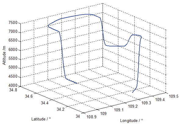
The flight trajectory of the aircraft was designed to reflect flexible and high-speed flying conditions for the purpose of performance evaluation. As shown in figure 3, there are different maneuvers such as level constant velocity motion, climbing, left turn, right turn, and diving involved in the flight process. The simulation parameters are shown in table 1. The simulation time was 1000 s; The filtering period was 1 s. The particle numbers in the PF and the numbers of Gaussian mixture components in the GMSPPF and RAGMSPPF were identical to those in the simulation case described in Section 4.1.
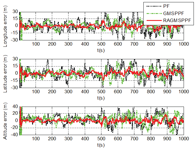
For the comparison analysis, simulation trials were conducted at the same conditions by the PF, GMSPPF and proposed RAGMSPPF, respectively. Further, in order to evaluate the performance of the proposed RAGMSPPF under the condition of different noises, the standard deviations of both system and measurement noises were enlarged to the twice of their initial values during the time period from 500 s to 1000 s.
Figure 4 illustrates the position error obtained by the PF, GMSPPF and proposed RAGMSPPF, respectively. As shown in figure 4, the errors in longitude, latitude and altitude by the PF are within the ranges of ± 19 m, ± 20 m and ± 22 m during the time period (100 s, 500 s) and within the ranges of ± 31 m, ± 33 m and ± 40 m during the time period (500 s, 1000 s). The GMSPPF improves the PF performance. The resultant errors in longitude, latitude and altitude by the GMSPPF are within the ranges of ± 16 m, ± 17 m and ± 20 m for the time period (100 s, 500 s) and within the ranges of ± 26 m, ± 27 m and ± 37 m for the time period (500 s, 1000 s). In contrast, the errors in longitude, latitude and altitude obtained by the RAGMSPPF are within the ranges of ± 9 m, ± 9 m and ± 10 m for the time period (100 s, 500 s) and within the ranges of ± 13 m, ± 14 m and ± 19 m for the time period (500 s, 1000 s), which are much smaller than those of the PF and GMSPPF. This demonstrates that the proposed RAGMSPPF can achieve much higher accuracy than the PF and GMSPPF.
Table 2 summarizes the mean absolute errors (MAE) and standard deviations (STD) of the PF, GMSPPF and proposed RAGMSPPF in the time periods (100 s, 500 s) and (500 s, 1000 s). It can be seen that the MAE and STD of the RAGMSPPF are much smaller than those of the other two filters. The above analysis demonstrates that the proposed RAGMSPPF outperforms the PF and GMSPPF, leading to improved accuracy for SINS/SAR integrated navigation.
Conclusions
This paper presents a new RAGMSPPF by absorbing the merits of the GMSPPF and robust adaptive estimation. This method approximates state mean and covariance via Sigma-point transformation combined with new measurement information. It enables the adjustment of state mean and covariance via the equivalent weight function and adaptive factor to effectively restrain the disturbances of singular measurements and system noise on state estimation. It also provides more efficient predicted prior and posterior density functions for time and measurement updates, thus more suitable for the filtering calculation of a nonlinear and non-Gaussian model. Simulations and comparison analysis demonstrate that the proposed RAGMSPPF outperforms the PF and GMSPPF, leading to improved accuracy for SINS/SAR integrated navigation.
Future research work will focus on improvement of the proposed RAGMSPPF. The proposed RAGMSPPF will be combined with the advanced artificial intelligence technologies such as pattern recognition, neural network and advanced expert systems, thus establishing an intelligent algorithm to automatically deal with the disturbances of various kinds of system error from different sources.
Acknowledgements
The work of this paper was supported by the National Natural Science Foundation of China (Project Number: 61174193) and the Specialized Research Fund for the Doctoral Program of Higher Education (Project Number: 20136102110036). It was also supported by the Australian Research Council (ARC) Discovery Early Career Award (DECRA) (DE130100274).
References
- Sebesta KD, Boizot N (2014) A Real-Time Adaptive High-Gain EKF, Applied to a Quadcopter Inertial Navigation System. IEEE Transactions on Industrial Electronics 61: 495-503.
- Simanek J, Reinstein M, Kubelka V (2015) Evaluation of the EKF-Based Estimation Architectures for Data Fusion in Mobile Robots. IEEE/ASME Transactions on Mechatronics 20: 985-990.
- Dahlin J, Lindsten F (2014) Particle filter-based Gaussian process optimisation for parameter inference. The International Federation of Automatic Control 8675-8680.
- Sedai S, Bennamoun M, Huynh du Q (2013) A Gaussian Process Guided Particle Filter for Tracking 3D Human Pose in Video. IEEE Trans Image Process 22: 4286-4300.
- Walker E, Rayman S, White RE (2015) Comparison of a particle filter and other state estimation methods for prognostics of lithium-ion batteries. Journal of Power Sources 287: 1-12.
- Uilhoorn FE (2014) A particle filter-based framework for real-time state estimation of a non-linear hyperbolic PDE system describing transient flows in CO2 pipelines. Computers & Mathematics with Applications 68: 1991-2004.
- Li Y, Zhao L, Coates M (2015) Particle flow auxiliary particle filter. IEEE International Workshop on Computational Advances in Multi-Sensor Adaptive Processing.
- Gonczarek A, Tomczak JM (2016) Articulated tracking with manifold regularized particle filter. Machine Vision and Applications 27: 275-286.
- Ito K, Xiong K (2000) Gaussian filters for nonlinear filtering problems. IEEE Transactions on Automatic Control 45: 910-927.
- Merwe RV, Doucet A, Freitas ND, et al. (2001) The Unscented Particle Filter. Advances in Neural Information Processing Systems 13: 584-590.
- Merwe RV, (2004) Sigma-Point Kalman Filters for Probabilistic Inference in Dynamic State-Space Models. OGI School of Science & Engineering at Oregon Health & Science University.
- Miroslav S, Dunik JR (2005) Sigma Point Gaussian Sum Filter Design Using Square Root Unscented Filters, 16th IFAC World Congress.
- Kotecha JH, Djurić PM (2003) Gaussian sum particle filtering. IEEE Transactions on Signal Processing 51: 2602-2612.
- Kotecha JH, Djurić PM (2003) Gaussian particle filtering. IEEE Transactions on Signal Processing 51: 2592-2601.
- Alspach DL, Sorenson HW (1972) Nonlinear Bayesian estimation using Gaussian sum approximations. IEEE Transactions on Automatic Control 17: 439-448.
- Yang YX (2006) Adaptive Navigation and Kinematic Positioning. Beijing: Sino Maps Press.
- Zhou JW (1989) Classical error theory and robust estimation. Acta Geoda et Cartographica Sinica 18: 115-120.
- Huber PJ, Ronchehi EM (2009) Robust Statistics. (2nd edn) John Wiley & Sons, New York, 46-67.
- Terejanu G, Singla P, Singh T, et al. (2008) A novel Gaussian Sum Filter Method for accurate solution to the nonlinear filtering problem. International Conference on Information Fusion 1-8.
- Zhong YM, Gao SS, Li W (2012) A quaternion-based method for SINS/SAR integrated navigation system. IEEE Transactions on Aerospace and Electronic Systems 48: 514-524.
Corresponding Author
Yongmin Zhong, Associate Professor, School of Engineering, Department of Aerospace, Mechanical and Manufacturing Engineering, RMIT University, Bundoora, VIC 3083, Australia, Tel: +61-3-99256018.
Copyright
© 2016 Yan H, et al. This is an open-access article distributed under the terms of the Creative Commons Attribution License, which permits unrestricted use, distribution, and reproduction in any medium, provided the original author and source are credited.

