The Outcome of an Engineering Undertaking of Importance Must be Quantified to Assure its Success and Safety: Review

Abstract

The outcome a of crucial engineering undertaking must be quantified at the design/planning stage to assure its success and safety, and since the probability of an operational failure is, in effect, never zero, such a quantification should be done on the probabilistic basis. Some recently published work on the probabilistic predictive modeling (PPM) and probabilistic design for reliability (PDfR) of aerospace electronic and photonic (E&P) products, including human-in-the-loop (HITL) problems and challenges, is addressed and briefly reviewed. The effort was lately "brought down to earth" to model possible collision in automated driving (AD). In addition, some problems and tasks beyond the E&P and vehicular engineering field are also addressed with an objective to show how the developed methods and approached can be effectively and fruitfully employed, whenever there is a need to quantify the reliability of an engineering technology with consideration of the human performance.

Accordingly, the following nine problems have been addressed in this review with an objective to show how the outcome of a critical engineering endeavor can be predicted using PPM and PDfR concept: 1) Accelerated testing in E&P engineering: significance, attributes and challenges; 2) Failure-oriented accelerated testing (FOAT), its objective and role; 3) PPM approach and PDfR concept, their roles and applications; 4) Kinetic multi-parametric Boltzmann-Arrhenius-Zhurkov (BAZ) equation as the "heart" of the PDfR concept; 5) Burn-in-testing (BIT) of E&P products with an attempt to shed light on the basic "to BIT or not to BIT" question; 6) Adequate trust is an important constituent of the human-capacity-factor (HCF) affecting the outcome of a mission or an extraordinary situation; 7) PPM of an emergency-stopping situation in automated driving (AD) or on a railroad (RR); 8) Quantifying the astronaut's/pilot's/driver's/machinist's state of health (SoH) and its effect on his/hers performance; 9) Survivability of species in different habitats. The objective of the latter effort is to demonstrate that the developed PPM approaches and methodologies, and particularly those using multiparametric BAZ equation, could be effectively employed well beyond the vehicular engineering area.

The general concepts are illustrated by numerical examples. All the considered PPM problems were treated using analytical ("mathematical") modeling. The attributes of the such modeling, the background of the multiparametric BAZ equation and the ten major principles ("the ten commandments") of the PDfR concept are addressed in the appendices.

Acronyms

AD: Automated Driving; ASD: Anticipated Sight Distance; BAZ: Boltzmann-Arrhenius-Zhurkov (equation); BGA: Ball Grid Array; BIT: Burn-in Testing; BTC: Bathtub Curve; CTE: Coefficient of Thermal Expansion; DEPDF: Double-Exponential Probability Distribution Function; DfR: Design for Reliability; E&P: Electronic and Photonic; FOAT: Failure-Oriented-Accelerated-Testing; FoM: Figures of Merit; HALT: Highly-Accelerated-Life-Testing; HCF: Human Capacity Factor; HE: Human Error; HF: Human Factor; HITL: Human-in-the-Loop; IMP: Infant Mortality Portion (of the BTC); MTTF: Mean-Time-to-Failure; MWL: Mental Workload; NIH: "Not invented here"; PAM: Probabilistic Analytical Modeling; PDF: Probability Distribution Function; PDfR: Probabilistic Design for Reliability; PHM: Prognostics and Health Monitoring; PPM: Probabilistic Predictive Modeling; PRA: Probabilistic Risk Analysis; QT: Qualification Testing; RR: Railroad; RUL: Remaining Useful Life; SAE: Society of Automotive Engineers; SF: Safety Factor; SJI: Solder Joint Interconnections; SoH: State of Health; SFR: Statistical Failure Rate; TTF: Time-to-Failure

Introduction

Quo vadis?

St. Paul

Progress in vehicular safety is achieved today mostly through various, predominantly experimental and posteriori- statistical, ways to improve the hard- and software of the instrumentation and equipment, implement better ergonomics, and introduce and advance other more or less well established efforts of experimental reliability engineering and traditional human psychology that directly affect product's reliability and human performance. There exists, however, a significant potential for the reduction in accidents and casualties in aerospace, maritime, automotive and railroad engineering through better understanding the role that various uncertainties play in the planner's and operator's worlds of work, when never failure-free navigation equipment and instrumentation, never hundred percent predictable response of the object of control (air- or spacecraft, a car, a train, or an ocean-going vessel), uncertain-and-often-harsh environment and never-perfect human performance contribute jointly to the outcome of a vehicular mission or an extraordinary situation. By employing quantifiable and measurable ways of assessing the role and significance of critical uncertainties and treating HITL as a part, often the most crucial part, of a complex man-instrumentation-vehicle-environment-navigation system and its critical interfaces, one could improve dramatically the state-of-the-art in assuring operational safety of a vehicle and its passengers and crew. This can be done by predicting, quantifying and, if necessary and possible, even specifying an adequate (typically low enough, but different for different vehicles, missions and circumstances) probability of success and safety of a mission or an off-normal situation [1-19].

Nothing and nobody is perfect, and the difference between a highly reliable technology, object, product, performance or a mission and an insufficiently reliable one is "merely" in the levels of their never-zero probability of failure. Application of the PPM approach and the PDfR concept [20-31] provide a natural and an effective means for reduction of vehicular casualties. This approach, as has been indicated, can be applied also beyond the vehicular field, in devices whose operational reliability is critical, such as, e.g., military, long-haul communications systems or medical devices [32]. When success and safety of a critical undertaking are imperative, ability to predict and quantify its outcome is paramount. The application of the PDfR concept can improve dramatically the state-of-the-art in reliability and quality engineering by making the art of creating reliable products and assure adequate human performance into a well substantiated and "reliable" science. Tversky and Kahneman (1979 Nobel Memorial Prize in Economics) [33] where, perhaps, the first who indicated the importance of considering the role of uncertainties in decision making and, particularly, in analyzing the role of cognitive biases that affect decision making in life and work. Since, however, these investigators were, although outstanding, but traditional human psychiatrists, no quantitative, not to mention probabilistic, assessments, were suggested.

It should be pointed out that while the traditional statistical human-factor-oriented approaches are based mostly on experimentations followed by statistical analyses, an important feature of the PDfR concept is that it is based upon, and start with, a physically meaningful and flexible predictive model (such as the BAZ one) geared to the appropriate FOAT [34-37]. Statistics and/or experimentation can be applied afterwards, to establish the important numerical characteristics of the selected model (such as, say, the mean value and the standard deviation in a normal distribution) and/or to confirm the suitability of a particular model for the application of interest. The highly-focused and highly cost-effective FOAT, the "heart" of the PDfR concept, is aimed, first of all, at understanding and/or at confirming the anticipated physics of failure (see Table 1 below). The traditional, about forty-years-old, highly accelerated life testing (HALT), although sheds important light on the reliability of the E&P product of interest (bad things would not last for forty years, would they?), does not quantify reliability and, because of that could hardly improve our understanding of the device's and/or package's physics of failure. FOAT, geared to a physically meaningful PDfR model, can be used as an appropriate extension and modification of HALT. An important attribute of the PPM/PDfR/FOAT based approach is if the predicted probability of non-failure, based on the applied PDfR methodology and FOAT effort, is, for whatever reason, not acceptable, then an appropriate sensitivity analysis (SA) using the already developed and available algorithms and calculation procedures can be effectively conducted to improve the situation without resorting to additional expensive and time-consuming testing.

Such a cost-effective and insightful approach is applicable, with the appropriate modifications and generalizations, if necessary, to numerous, not even necessarily in the vehicular domain, when a human-in-control encounters an uncertain environment or a hazardous situation. The suggested quantification-based HITL approach is applicable also when there is an incentive to quantify human's qualifications and/or when there is a need to assess and possibly improve human performance and possible role in a particular engagement.

An important additional consideration in favor of quantification of the reliability has to do with the always desirable optimizations. The best engineering product is, in effect, as is known, the best compromise between the requirements for its reliability, cost effectiveness and time-to-market (to completion). The latter two requirements are always quantified. No effective optimization could be achieved, of course, if reliability is not optimized as well. In the HITL situations, such an optimization should be done considering the role of the human factor.

In the review that follows some important problems and tasks associated with assuring success and safety of vehicular and other engineering undertakings are addressed with an objective to show what could and should be done differently, when high reliability is imperative, and should be quantified to assure its adequate level and cost effectiveness. A simple example on how to optimize reliability [38] indicates that optimization of reliability can be achieved by optimizing the product's availability - the probability that the product is sound, i.e. available to the user, when needed. When encountering a particular reliability problem at the design, fabrication, testing, or an operation stage of the product's life, and considering the use of predictive modeling to assess the seriousness and the likely consequences of its detected failure, one has to choose whether a statistical, or a physics-of-failure-based, or a suitable combination of these two major modeling tools should be employed to address the problem of interest and to decide on how to proceed.

A three-step concept (TSC) is suggested as a possible way to go in such a situation [39,40]. The classical statistical Bayes formula can be used at the first step as a technical diagnostics tool, with an objective is to identify, on the probabilistic basis, the faulty (malfunctioning) device(s) from the obtained signals ("symptoms of faults"). The multi-parametric BAZ model can be employed at the TSC's second step to assess the remaining useful life (RUL) of the faulty device(s). If the assessed RUL is still long enough, no action might be needed, but if it is not, corrective restoration action becomes necessary. In any event, after the first two steps are carried out, the device is put back into operation, provided that the assessed probability of its continuing failure-free operation is found to be satisfactory. If failure nonetheless occurs, the third step should be undertaken to update reliability. Statistical beta-distribution, in which the probability of failure itself is treated as a random variable, is suggested to be used at this step. The suggested concept is illustrated by a numerical example geared to the use of the prognostics-and-health-monitoring (PHM) effort in actual operation, such as, e.g., en-route flight mission.

The major principles of an analytical modeling approach, the background and the attributes of the BAZ equation [41-44] and the major principles of the PDfR concept are summarized in Appendix A, Appendix B and Appendix C (the latter - in the form of "the ten commandments"), respectively.

Review

Accelerated testing in electronics and photonics: Significance, attributes and challenges

"Golden rule of an experiment: The duration of an experiment should not exceed the lifetime of the experimentalist".

Unknown experimental physicist

Accelerated testing is both a must and a powerful tool in E&P manufacturing. This is because getting maximum reliability information in minimum time and at minimum cost is the major goal of an E&P manufacturer, but also because it is impractical to wait for failures, when the lifetime of a typical today's E&P product manufactured using the existing "best practices" is hundreds of thousands of hours, regardless of whether this lifetime is or is not be predicted with sufficient accuracy. Different types of accelerated tests in today's E&P engineering are summarized in Table 1.

A typical example of product development testing (PDT) is shear-off testing conducted when there is a need to determine the most feasible bonding material and its thickness, and/or to assess its bonding strength and/or to evaluate the shear modulus of the material. HALT is currently widely employed, in different modifications, with an intent to determine the product's reliability weaknesses, assess its reliability limits, and ruggedize the product by applying elevated stresses (not necessarily mechanical and not necessarily limited to the anticipated field stresses) that could cause field failures, and to provide supposedly large (although, actually, unknown) safety margins over expected in-use conditions. HALT often involves step-wise stressing, rapid thermal transitions, and other means that enable to carry out testing in a time- and cost- effective fashion. HALT is a "discovery" test. It is not a qualification test (QT) though, i.e. not a "pass/fail" test. It is the QT that is the major means for making a viable E&P device or package into a justifiably marketable product. While many HALT aspects are different for different manufacturers and often kept as proprietary information, QTs and standards are the same for the given industry and product type. Burn-in testing (BIT) is a post-manufacturing test. Mass fabrication, no matter how good the design effort and the fabrication technologies are, generates, in addition to desirable and relatively robust ("strong") products, also some undesirable and unreliable ("weak") devices ("freaks"), which, if shipped to the customer, will most likely fail in the field. BIT is supposed to detect and to eliminate such "freaks". As a result, the final bathtub curve (BTC) of a product that underwent BIT is not expected to contain the infant mortality portion (IMP). In the today's practice BIT, a destructive test for the "freaks" and a non-destructive for the healthy devices, is often run within the framework of, and concurrently with, HALT.

Are the today's practices based on the above accelerated testing adequate? A funny, but quite practical, definition of a sufficiently robust E&P product is that "reliability it is when the customer comes back, not the product". It is well known, however, that E&P products that underwent HALT, passed the existing QTs and survived BIT often prematurely fail in the field. So, what could and should be done differently?

Failure-oriented-accelerated-testing (FOAT), its objective and role

"Say not, "I have found the truth," but rather, "I have found a truth."

Kahlil Gibran, Lebanese artist, poet and writer

One crucial shortcoming of the today's E&P reliability assurance practices is that they are seldom based on good understanding the underlying reliability physics for the particular E&P product, but most importantly, although claim its lifetime, do not suggest a trustworthy effort to quantify it. A possible way to go is to design and conduct FOAT aimed, first of all, at understanding and confirming the anticipated physics of failure, but also on using the FOAT data to predict the operational reliability of the product (last column in Table 1). To do that, FOAT should be geared to an adequate, simple, easy-to-use and physically meaningful predictive model. BAZ (see Appendix B and section 3 below) model can be employed in this capacity.

Predictive modeling has proven for many years to be a highly useful and a highly time- and cost-effective means for understanding the physics of failure in reliability engineering, as well as for designing the most effective accelerated tests. It has been recently suggested that a highly focused (on the most vulnerable material and/or structural element of the design, such as, e.g., solder joint interconnections) and, to an extent possible, highly cost effective FOAT is considered as the experimental basis, the "heart", of the new fruitful, flexible and physically meaningful design-for-reliability concept - PDfR (see next section for details). FOAT should be conducted in addition to, and, in some cases, even instead of, HALT, especially when developing new technologies and for new products, whose operational reliability is, as a rule, unclear and for which no experience is accumulated yet and no best practices nor suitable HALT methodologies are not yet developed. Quantitative estimates based on the FOAT and subsequent PPM might not be perfect, at least at the beginning, but it is still better to pursue this effort rather than to turn a blind eye on the never-zero probability of the product's failure and that the reliability of an E&P product cannot be assured, if this probability is not assessed and made adequate for the given product. If one sets out to understand the physics of failure to create, in accordance with the "principle of practical confidence", a failure-free product, conducting FOAT is imperative to confirm the usage of a particular predictive model, such as BAZ equation, to confirm the physics of failure, and establish the numerical characteristics (activation energy, time constant, sensitivity factors, etc.) of the selected model.

FOAT could be viewed as an extension of HALT, but while HALT is a "black box", i.e., a methodology which can be perceived in terms of its inputs and outputs without clear knowledge of the underlying physics and the likelihood of failure, FOAT is a "transparent box", whose objective is to confirm the use of a particular reliability model. While HALT does not measure (does not quantify) reliability, FOAT does. The major assumption is, of course, that this model should be valid for both accelerated and actual operation conditions. HALT that tries to "kill many unknown birds with one (also not very well known) stone" has demonstrated, however, over the years its ability to improve robustness through a "test-fail-fix" process, in which the applied stresses (stimuli) are somewhat above the specified operating limits. This "somewhat above" is based, however, on an intuition, rather than on a calculation.

There is a general, and, to great extent, justified, perception that HALT is able to precipitate and identify failures of different origins. HALT can be used therefore for "rough tuning" of product's reliability, and FOAT could be employed when "fine tuning" is needed, i.e., when there is a need to quantify, assure and even specify the operational reliability of a product. The FOAT based approach could be viewed as a quantified and reliability physics oriented HALT. The FOAT approach should be geared to a particular technology and application, with consideration of the most likely stressors. FOAT and HALT could be carried out separately, or might be partially combined in a particular AT effort. New products present natural reliability concerns, as well as significant challenges at all the stages of their design, manufacture and use. An appropriate combination of HALT and FOAT efforts could be especially useful for ruggedizing and quantifying reliability of such products. It is always necessary to correctly identify the expected failure modes and mechanisms, and to establish the appropriate stress limits of HALTs and FOATs with an objective to prevent "shifts" in the dominant failure mechanisms. There are many ways of how this could be done. E.g., the test specimens could be mechanically pre-stressed, so that the temperature cycling could be carried out in a more narrow range of temperatures [45]. But a better way seems to be replacement of temperature cycling with a more cost-effective, less time consuming and, most importantly, more physically meaningful accelerated test, such as low-temperature/random-vibrations bias (see section 4.3).

PPM approach and PDfR concept, their roles and applications

"A pinch of probability is worth a pound of perhaps."

James G. Thurber, American writer and cartoonist

Design for reliability (DfR) is, as is known, a set of approaches, methods and best practices that are supposed to be used at the design stage of a product to minimize the risk that the fabricated product might not meet the reliability objectives and customer expectations. When deterministic approach is used, the safety factor (SF) is defined as the ratio $SF=\frac{C}{D}$ of the capacity ("strength") C of the product to the demand ("stress") D. When PDfR approach is considered, the SF can be introduced as the ratio $SF=\frac{\prec \psi \succ }{\widehat{s}}$ of the mean value $\prec \psi \succ$ of the safety margin SM = Ψ = C - D to its standard deviation $\widehat{s}$. In this analysis, having in mind the application of the BAZ equation, the probability P of non-failure is used as the suitable measure of the product's reliability. Here are several simple PDfR practical examples.

Reliable seal glass bond in a ceramic package design: AT&T ceramic packages fabricated at its Allentown (former "Western Electric") facility in mid-nineties experienced numerous failures during accelerated tests. It has been determined that this happened because the seal/solder glass that bonded two ceramic parts had a higher coefficient of thermal expansion (CTE) than the ceramic lid and substrate, and therefore, when the packages were cooled down from the high manufacturing temperature of about 800-900 ℃ to the room temperature, all the packages cracked. To design a reliable seal we had not only to replace the existing seal glass with a glass material that would have a lower CTE than the ceramics, but, in addition to that, we had to make sure that the interfacial shearing stresses at the ceramics/glass interfaces subjected to compression at low temperatures would be low enough not to crack the seal glass material. Treating the CTE's of the brittle ceramic and brittle glass materials as normally distributed random variables, the following PDfR methodology was developed and applied. No failures were observed in the manufactured packages, designed and manufactured based on the developed methodology. Here is how a reliable seal glass material was selected in a ceramic IC package using this PDfR approach [46].

The maximum interfacial shearing stress in a thin solder glass layer in a ceramic package design can be computed as τmax = khgσmax. Here $k=\sqrt{\frac{\lambda }{\kappa }}$ is the parameter of the interfacial shearing stress, $\lambda =\frac{1-v_c}{E_c{h}_c}+\frac{1-v_g}{E_g{h}_g}$ is the axial compliance of the assembly, $\kappa =\frac{h_c}{3G_c}+\frac{h_g}{3G_g}$ is its interfacial compliance, $G_c=\frac{E_c}{2\left(1+v_c\right)},G_g=\frac{E_g}{2\left(1+v_g\right)}$ are the shear moduli of the ceramics and glass materials, ${\sigma }_{\max }=\frac{△\alpha \Delta t}{\lambda h_g}$ is the maximum normal stress in the mid-portion of the glass layer, ∆t is the change in temperature from the soldering temperature to the low (room or testing) temperature, $\Delta \alpha ={\overline{\alpha }}_c-{\overline{\alpha }}_g$ is the difference in the effective CTEs of the ceramics and the glass, ${\overline{\alpha }}_{c,g}=\frac{1}{\Delta t}{\displaystyle \underset{t}{\overset{t_0}{\int }}{\alpha }_{c,g}\left(t\right)dt}$ are these coefficients for the given temperature t, t₀ is the annealing (zero stress, setup) temperature, and α_c,g(t) are the time dependent CTEs for the materials in question. In an approximate analysis one could assume that the axial compliance λ of the assembly is due to the glass only, so that $\lambda \approx \frac{1-v_g}{E_g{h}_g}$ and therefore the maximum normal stress in the solder glass can be evaluated as ${\sigma }_{\max }=\frac{E_g}{1-v_g}\Delta \alpha \Delta t$. While the geometric characteristics of the assembly, the change in temperature and the elastic constants of the materials can be determined with high accuracy, this is not the case for the difference in the CTEs of the brittle materials of the glass and the ceramics. In addition, because of the obvious incentive to minimize this difference, such a mismatch is characterized by a small difference of close and appreciable numbers. This contributes to the uncertainty of the problem and makes PPM necessary. Treating the CTEs of the two materials as normally distributed random variables, we evaluate the probability P that the thermal interfacial shearing stress is compressive (negative) and, in addition, does not exceed a certain allowable level [9]. This stress is proportional to the normal stress in the glass layer, which is, in its turn, proportional to the difference $\Psi ={\alpha }_c-{\alpha }_g$ of the CTE of the ceramics and the glass materials. One wants to make sure that the requirement

$0\le \Psi \le {\Psi }_{*}=\frac{{\sigma }_a}{E_g}\frac{1-{\nu }_g}{\Delta t}\text{ (1)}$

takes place with a high probability. For normally distributed random variables α_c and α_g the variable $\Psi ={\alpha }_c-{\alpha }_g$ is also normally distributed with the mean value and standard deviation as $\prec \psi \succ =\prec {\alpha }_c\succ -\prec {\alpha }_g\succ$ and $\sqrt{D_{\psi }}=\sqrt{D_c+D_g}$, where $\prec {\alpha }_c\succ$ and $\prec {\alpha }_g\succ$ are the mean values of the materials' CTEs, andD_candD_g are their variances. The probability that the above condition for the Ψ value takes place is

$P={\displaystyle \underset{0}{\overset{{\psi }_{*}}{\int }}{f}_{\psi }}(\psi )d\psi ={\Phi }_1({\gamma }^{*}-\gamma )-[1-{\Phi }_1(\gamma )]\text{ (2)}$

where

${\Phi }_1\left(t\right)=erft=\frac{1}{\sqrt{2\pi }}{\displaystyle \underset{-\infty }{\overset{t}{\int }}{e}^{-t^2/2}dt}\text{ (3)}$

is the error (Laplace) function, $\gamma =\frac{\prec \psi \succ }{\sqrt{D_{\psi }}}$ is the SF for the CTE difference and ${\gamma }^{*}=\frac{{\psi }^{*}}{\sqrt{D_{\psi }}}$ is the SF for the acceptable level of the allowable stress.

If, e.g., the elastic constants of the solder glass are E_g = 0.66 × 10⁶ kg/cm² and v_g = 0.27, the sealing (fabrication) temperature is 485 ℃ the lowest (testing) temperature is -65 ℃ (so that ∆t = 550 ℃), the computed effective CTE's at this temperature are $$_g = 6.75 × 10^-61/℃ and $$_c = 7.20 × 10^-61/℃, the standard deviations of these STEs are $\sqrt{D_c}=\sqrt{D_g}=0.25\times {10}^{-6}1/{}^{o}C$ and the (experimentally obtained) ultimate compressive strength for the glass material is σ_u = 5500 kg/cm², then, with the acceptable SF of, say, 4, we have σ* = σ_u/4 = 1375 kg/cm². The allowable level of the CTE parameter ψ = α_c - α_g is therefore

$${\psi }_{*}=\frac{{\sigma }_a}{E_g}\frac{1-v_g}{\Delta t}=\frac{1375}{0.66x{10}^6}\frac{0.73}{550}=2.765\times {10}^{-6}1/{}^{o}C,$$

and its calculated mean value $\prec \psi \succ$ and variance $D_{\psi }$ are $\prec \psi \succ =\prec {\alpha }_c\succ -\prec {\alpha }_g\succ =0.450\times {10}^{-6}\left(1/{}^{o}C\right)$ and $D_{\psi }=D_c+D_g=0.25\times {10}^{-12}\left(1/{}^{o}C\right)$. Then the predicted SFs are $\gamma =1.2726$ and ${\gamma }^{*}=7.8201$, and the corresponding probability of non-failure of the seal glass material is

$$P={\Phi }_1({\gamma }^{*}-\gamma )-[1-{\Phi }_1(\gamma )]=0.898$$

Note that if the standard deviations of the materials CTEs were only $\sqrt{D_c}=\sqrt{D_g}=0.1\times {10}^{-6}1/{}^{o}C$, then the SFs γ and γ*and the probability P of non-failure would be significantly higher: γ = 3.1825, γ* = 19.5556 and P = 0.999.

Application of extreme value distribution: An E&P device is operated in temperature cycling conditions. Let us assume that the random amplitude of the induced stress, when a single cycle of the random amplitude is applied, is distributed in accordance with the Rayleigh law, so that the probability density function of the random amplitude of the induced thermal stress is

$$f\left(r\right)=\frac{r}{D_x}\exp \left(-\frac{r^2}{2D_x}\right)\text{ (4)}$$

Here D_x is the variance of the distribution. Let us assess the most likely extreme value of the stress amplitude for a large number n of cycles.

The probability distribution density function g(y_n) and the probability distribution function G(y_n) for the extreme value Y_n of the stress amplitude are expressed as follows [28,47]:

$$g\left(y_n\right)=n{\left\{f\left(x\right){\left[F\left(x\right)\right]}^{n-1}\right\}}_{x=y_n}\text{ (5)}$$

and

$$G\left(y_n\right)={\left\{{\left[F\left(x\right)\right]}^n\right\}}_{x={\varsigma }_n}\text{ (6)}$$

respectively. Introducing the expression for the function G(y_n) into the expression for the function g(y_n), the following formula can be obtained for the probability density distribution function g(y_n):

$$g\left(y_n\right)=n{\varsigma }_n^2\exp \left(-\frac{{\varsigma }_n^2}{2}\right){\left[1-\exp \left(-\frac{{\varsigma }_n^2}{2}\right)\right]}^{n-1}\text{ (7)}$$

where ${\varsigma }_n=\frac{y_n}{\sqrt{D_x}}$ is the ratio of the sought amplitude after the loading is applied n times to the standard deviation of the random response in question. The condition g'(y_n) = 0 results in the equation:

${\varsigma }_n^2\left[n\exp \left(-\frac{{\varsigma }_n^2}{2}\right)-1\right]-\left[\exp \left(-\frac{{\varsigma }_n^2}{2}\right)-1\right]=0\text{ (8)}$

If the number n is large, the second term in this expression is small compared to the first term and can be omitted. Then we obtain: $n\exp \left(-\frac{{\varsigma }_n^2}{2}\right)-1=0.$ Hence,

$y_n={\varsigma }_n\sqrt{D_x}=\sqrt{2D_x\ln n}\text{ (9)}$

As evident from this result, the ratio of the extreme response y_n, after n cycles are applied, to the maximum response $\sqrt{D_x}$, when a single cycle is applied, is $\sqrt{2\ln n}$. This ratio is 3.2552 for 200 cycles, 3.7169 for 1000 cycles, and 4.1273 for 5000 cycles.

Adequate heat sink: Consider a heat-sink whose steady-state operation is determined by the Arrhenius equation (B-2) [28] (Appendix B). The probability of non-failure can be found using the exponential law of reliability as

$P=\exp \left[-\frac{t}{{\tau }_0}\exp \left(-\frac{U}{kT}\right)\right].\text{ (10)}$

Solving this equation for the absolute temperature T, we have:

$T=-\frac{U/k}{\ln \left(-\frac{{\tau }_0}{t}\ln P\right)}\text{ (11)}$

Addressing, e.g., a failure caused by the surface charge accumulation, for which the ratio of the activation energy to the Boltzmann's constant is $\frac{U}{k}=11600°K$, assuming that the FOAT- predicted time factor τ₀ is τ₀ = 2 × 10^-5 h, that the customer requires that the probability of failure at the end of the service time of t = 40,000 h is, say, Q = 10^-5, the obtained formula for the required temperature yields: T = 3523 °K = 79.3 ℃. Thus, the heat sink should be designed accordingly, and the product manufacturer should require that the vendor manufactures and delivers such a heat sink. The situation changes to the worse, if the temperature of the device changes, especially in a random fashion (see previous example 4.3.2), but this situation can also be predicted by a simple probabilistic analysis, which is, however, beyond the scope of this article.

Kinetic Multi-Parametric BAZ Equation as the "Heart" of the Pdfr Concept

"Everyone knows that we live in the era of engineering, however, he rarely realizes that literally all our engineering is based on mathematics and physics"

-Bartel Leendert van der Waerden, Dutch mathematician

Electronic package subjected to the combined action of two stressors

The rationale behind the BAZ equation is described in Appendix B. Let us consider, for the sake of simplicity, the action of just two stressors [49,50]: elevated humidity H and elevated voltage V. If the level I* of the leakage current is accepted as the suitable criterion of material/structural failure, then the equation (B-2) can be written as

$P=\exp \left[-{\gamma }_I{I}_{*}t\exp \left(-\frac{U_0-{\gamma }_{H}H-{\gamma }_{V}V}{kT}\right)\right]\text{ (12)}$

This equation contains four unknowns: The stress-free activation energy U₀, the leakage current sensitivity factor γ_I, the relative humidity sensitivity factor γ_H and the elevated voltage sensitivity factor γ_V. These unknowns can be determined experimentally, by conducting a three-step FOAT.

At the first step one should conduct the test for two temperatures, T₁ and T₂, while keeping the levels of the relative humidity H and the elevated voltage V unchanged. Assuming a certain level I* of the monitored/measured leakage current as the physically meaningful criterion of failure, recording during the FOAT the percentages P₁ and P₂ of non-failed samples, and using the above equation for the probability of non-failure, we obtain two equations for the probabilities of non-failure:

$P_{1,2}=\exp \left[-{\gamma }_I{I}_{*}{t}_{1,2}\exp \left(-\frac{U_0-{\gamma }_{H}H-{\gamma }_{V}V}{k{T}_{1.2}}\right)\right]\text{ (13)}$

where t₁ and t₂ are the testing times and T₁ and T₂ are the temperatures, at which the failures were observed. Since the numerators in these equations are the same, the following transcendental equation must be fulfilled:

$$f\left({\gamma }_I\right)=\ln \left(-\frac{\ln P_1}{I_{*}{t}_1{\gamma }_I}\right)-\frac{T_2}{T_1}\ln \left(-\frac{\ln P_2}{I_{*}{t}_2{\gamma }_I}\right)=0\text{ (14)}$$

This equation enables determining the leakage current sensitivity factor γ_I. At the second step, testing at two humidity levels, H₁ and H₂, should be conducted for the same temperature and voltage. This enables to determine the relative humidity sensitivity factor γ_H. Similarly, the voltage sensitivity factor γ_V can be determined, when testing is conducted at the third step at two voltage levels V₁ and V₂. The stress-free activation energy U₀ can be then evaluated from the above expression for the probability P of non-failure for any consistent combination of the relative humidity, voltage, temperature and time as

$$U_0={\gamma }_{H}H+{\gamma }_{V}V-kT\ln \left(-\frac{\ln P}{I_{*}t{\gamma }_I}\right)\text{ (15)}$$

If, e.g., after t₁ = 35 h of accelerated testing at the temperature of T₁ = 60 ℃ = 333 K, voltage V = 600 V and the relative humidity of H = 0.85, 10% of specimens reached the critical level I* = 3.5 μA of the leakage current and, hence, failed, then the corresponding probability of non-failure is P₁ = 0.9; and if after t₂ = 70 h of testing at the temperature T₂ = 85 ℃ = 358 K at the same relative humidity and voltage levels, 20% of the tested samples failed, so that the probability of non-failure is P₂ = 0.8, then the factor γ_I can be found from the equation

$$f\left({\gamma }_I\right)=\ln \left(\frac{0.10536}{{\gamma }_I}\right)-1.075075\ln \left(-\frac{0.22314}{{\gamma }_I}\right)=0$$

Its solution is γ_I = 4926 ^-1 (μA)^-1, so that γ_I I* = 17,241 ^-1. Tests at the second step are conducted for two relative humidity levels H₁ and H₂ while keeping the temperature and the voltage unchanged. Then the factor γ_H can be found as:

$${\gamma }_H=\frac{kT}{H_1-H_2}\left[\ln \left(-0.5800x{10}^{-4}\frac{\ln P_1}{t_1}\right)-\ln \left(-0.5800x{10}^{-4}\frac{\ln P_2}{t_2}\right)\right]$$

If, e.g., 5% of the tested specimens failed after t₁ = 40 h of testing at the relative humidity of H₁ = 0.5, at the voltage V = 600 V and at the temperature T = 60 ℃ = 333 K ( P₁ = 0.95), and 10% of the specimens failed ( P₂ = 0.9), after t₂ = 55 h of testing at this temperature, but at the relative humidity of H₂ = 0.85, then the above expression yields: γ_H = 0.03292 eV. At the third step, when testing at two voltage levels V₁ = 600 V and V₂ = 1000 V is carried out for the same temperature-humidity bias at T = 85 ℃ = 358 K and H = 0.85, and 10% of the specimens failed after t₁ = 40 h ( P₁ = 0.9), and 20% of the specimens failed after t₂ = 80 h of testing ( P₂ = 0.8), then the factor γ_V for the applied voltage and the predicted stress-free activation energy U₀ are as follows:

$${\gamma }_V=\frac{0.02870}{400}\left[\ln \left(-0.5800x{10}^{-4}\frac{\ln P_2}{t_2}\right)-\ln \left(-0.5800x{10}^{-4}\frac{\ln P_1}{t_1}\right)\right]=4.1107x{10}^{-6}eV/V$$

and

$\begin{array}{l}{U}_0={\gamma }_H{H}_1+{\gamma }_V{V}_1-k{T}_1\ln \left(-\frac{\ln P_1}{I_{*}{t}_1{\gamma }_I}\right)=0.03292x0.5+4.1107x{10}^{-6}x600-\\ -8.61733x{10}^{-5}x358\ln \left(-\frac{\ln 0.9}{3.5x35x4893.2}\right)=-0.01646+0.00247+0.47984=0.4988eV\end{array}$

No wonder that the third term in this equation plays the dominant role. It is noteworthy, however, that external loading may also have an effect on the "stress-free" activation energy. The author intends to investigate such a possibility as a future work.

The activation energy U₀ in the above numerical example (with the rather tentative, but still realistic, input data) is about U₀ = 0.5 eV. This result is consistent with the existing reference information. This information (Bell Labs data) indicates that for failure mechanisms typical for semiconductor devices the stress-free activation energy ranges from 0.3 eV to 0.6 eV, for metallization defects and electro-migration in Al it is about 0.5 eV, for charge loss it is on the order of 0.6 eV, for Si junction defects is 0.8 eV. Other known activation energy values used in E&P reliability engineering assessments are more or less on the same order of magnitude. (See also http://nomtbf.com/2012/08/where-does-0-7ev-come-from). With the above information, the following expression for the probability of non-failure can be obtained:

$$P\text{ =}\text{exp}\left[-172410t\exp \left(-\frac{0.4988-0.03292H-4.1107\times {10}^{-6}V}{8.61733\times {10}^{-5}T}\right)\right]$$

If, e.g., t = 10 h, H = 0.20, V = 220 V, and the operation temperature is T = 70 ℃ = 343 K, then the probability of non-failure at these conditions is

$$\text{P = exp[-172410 exp}\left(-\frac{0.4990\text{ - 0}\text{.0066 - 0}\text{.0009}}{0.02956}\right)\text{] = 0}\text{.9897}\text{.}$$

Clearly, the TTF is not an independent characteristic of the lifetime of a product, but depends on the predicted or specified probability of its failure. If this probability is high, the lifetime of the product is short, and vice versa, if the probability of non-failure is low, the corresponding lifetime is long.

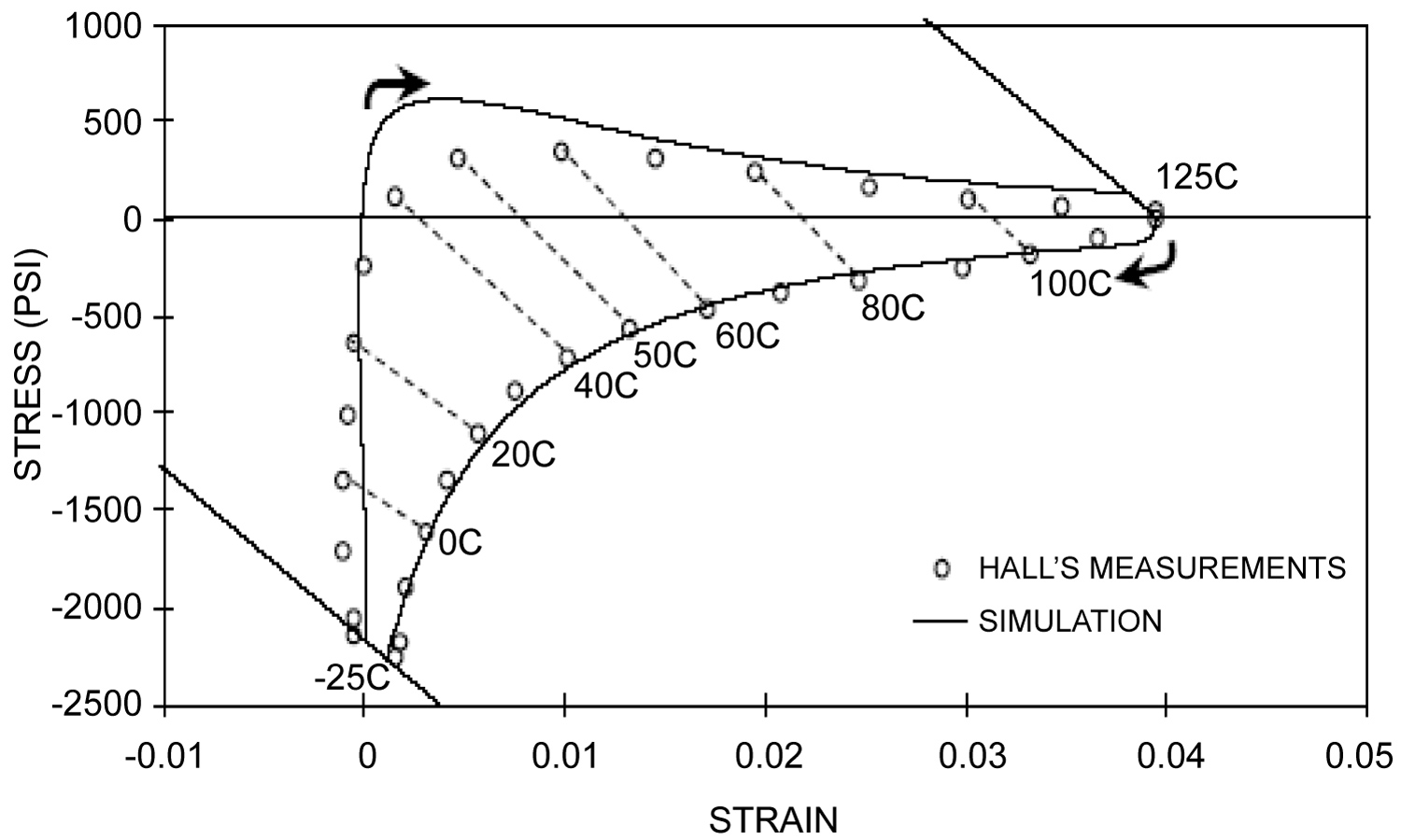
Predicted lifetime of SJIs: Application of Hall's concept

Using the BAZ model (see Appendix B), the probability of non-failure of the SJI experiencing inelastic strains during temperature cycling [48-53] can be sought as

$P=\exp \left[-\gamma Rt\exp \left(-\frac{U_0-nW}{kT}\right)\right].\text{ (16)}$

Here U₀ is the activation energy and is the characteristic of the propensity of the solder material to fracture, W is the damage caused in the solder material by a single temperature cycle and measured, in accordance with Hall's concept [50-53], by a hysteresis loop area of a single temperature cycle for the strain of interest, T is the absolute temperature (say, the mean temperature of the cycle), n is the number of cycles, k is Boltzmann's constant, t is time, R, Ω is the measured (monitored) electrical resistance at the joint location, and γ is the sensitivity factor for the measured electrical resistance.

The above equation for the probability of non-failure makes physical sense. Indeed, this probability is "one" at the initial moment of time, when the electrical resistance of the solder joint structure is next-to-zero. This probability decreases with time because of the material aging and structural degradation, and even not necessarily only because of temperature cycling leading to crack initiation and propagation. The probability of non-failure is lower for higher electrical resistance (a resistance as high as, say, 450 Ω, can be viewed as an indication of an irreversible mechanical failure of the joint). Materials with higher activation energy U₀ are characterized by higher fracture toughness and have a higher probability of non-failure. The increase in the number n of cycles leads to lower effective energy U = U₀ - nW, and so does the energy W of a single cycle (Figure 1).

It could be shown (see Appendix B) that the maximum entropy of the above probability distribution takes place at the MTTF expressed as:

$\tau =\frac{1}{\gamma R}\exp \left(-\frac{U_0-nW}{kT}\right).\text{ (17)}$

Mechanical failure, because of temperature cycling, takes place, when the number n of cycles is $n_f=\frac{U_0}{W}.$ When failure occurs, the temperature in the denominator in the parenthesis in the equation for the MTTF τ becomes irrelevant. In this case the measured probability of non-failure for the situation, when failure takes place, is

$P_f=\exp \left(\frac{t_f}{{\tau }_f}\right).\text{ (18)}$

Here ${\tau }_f=\frac{1}{\gamma R_f}$ is the MTTF. If, e.g., 20 specimens were temperature cycled and the high resistance R_f = 450 Ω considered as an indication of material's failure, was detected in 75 of them, then the probability of non-failure is P_f = 0.25. If the number of cycles during such FOAT was, e.g., n_f = 2000, and each cycle lasted, say, for 20 min =1200 sec., then the predicted time-to-failure TTF is t_f = 2000 × 1200 = 24 × 10⁵ sec, the sensitivity factor γ for the electrical resistance is

$\gamma =\frac{-\ln P_f}{R_f{t}_f}=\frac{-\ln 0.25}{450x24x{10}^5}=1.2836x{10}^{-9}{\Omega }^{-1}{\sec }^{-1};$

and the predicted MTTF is

${\tau }_f=\frac{1}{1.2836x{10}^{-9}x450}\sec =480.9hrs=20.0days.$

According to Hall's concept [51-54] the energy of a single cycle should be evaluated by running a special test, in which appropriate strain gages should be used. Let, e.g., in these tests the area of the hysteresis loop of a single cycle was W = 2.5 × 10^-4 eV. Then the stress-free activation energy of the solder material is U₀ = nfW = 2000 × 2.5 × 10^-4 = 0.5 eV. In order to assess the number of cycles to failure in actual operation conditions one could assume that the temperature range in these conditions is, say, half the accelerated test range, and that the area W of the hysteresis loop is proportional to the temperature range. Then the number of cycles to failure is

$n_f=\frac{U_0}{W}=\frac{0.5}{2.5x{10}^{-4}}=2000.$

If the duration of one cycle is one day, then the predicted TTF is t_f = 2000 days = 5.48 years.

Accelerated testing based on temperature cycling should be replaced

It is well known that it is the combination of low temperatures and repetitive dynamic loading that accelerate dramatically the propagation of fatigue cracks, whether elastic or inelastic. A modification of the BAZ model is suggested [48,49] for the evaluation of the lifetime of SJIs experiencing inelastic strains. The experimental basis of the approach is FOAT. The test specimens were subjected to the combined action of low temperatures (not to elevated temperatures, as in the classical Arrhenius model) and random vibrations with the given input energy spectrum of the "white noise" type. The methodology suggested and employed in [48,49] is viewed as a possible, effective and attractive alternative to temperature cycling, which is, as is well known, costly, time- and labor- consuming and often even misleading accelerated testing approach. This is because the temperature range in accelerated temperature cycling has to be substantially wider than what the material will most likely encounter in actual use conditions, and properties of E&P materials are, as is known, temperature sensitive.

As long as inelastic deformations take place, it is assumed that it is these deformations (which typically occur at the peripheral portions of the soldered assembly, where the interfacial stresses are the highest) determine the fatigue lifetime of the solder material, and therefore the state of stress in the elastic mid-portion of the assembly does not have to be accounted for. The roles of the size and stiffness of this mid-portion have to be considered, however, when determining the very existence and establishing the size of the inelastic zones at the peripheral portions of the soldered assemblies. Although the detailed numerical example has been carried out for a ball-grid-array (BGA) design, it is applicable also to highly popular today column-grid-array (CGA) and quad-flat-nolead (QFN) designs, as well as to, actually, any packaging design. It is noteworthy in this connection that it is much easier to avoid inelastic strains in CGA and QFN structures than in the actually tested BGA design.

Random vibrations were considered in the developed methodology as a white noise of the given ratio of the acceleration amplitudes squared to the vibration frequency. Testing was carried out for two PCBs, with surface-mounted packages on them, at the same level (with the mean value of 50 g) of three-dimensional random vibrations. One board was subjected to the low temperature of -20 ℃ and another one - to -100 ℃. It has been found, by preliminary calculations that the solder joints at -20 ℃ will still perform within the elastic range, while the solder joints at -100 ℃ will experience inelastic strains. No failures were detected in the joints of the board tested at -20 ℃, while the joints of the board tested at -100 ℃ failed after several hours of testing.

Predicted "static fatigue" lifetime of an optical silica fiber

BAZ equation can be effectively employed as an attractive replacement of the widely used today purely empirical power law relationship for assessing the "static fatigue" (delayed fracture) lifetime of optical silica fibers [41]. The literature dedicated to delayed fracture of ceramic and silica materials, mostly experimental, is enormous. In the analysis below the combined action of tensile loading and an elevated temperature is considered.

Let, e.g., the following input information is obtained at the FOAT first step for a polyimide coated fiber intended for elevated temperature operations: 1) After t₁ = 10 h of testing at the temperature of T₁ = 300 ℃ = 573 °K, under the stress of σ = 420 kg/mm², 10% of the tested specimens failed, so that the probability of non-failure is P₁ = 0.9; 2) After t₂ = 8.0 h of testing at the temperature of T₂ = 350 ℃ = 623 °K under the same stress, 25% of the tested samples failed, so that the probability of non-failure is P₂ = 0.75. Forming the equation for the probability of non-failure in accordance with the BAZ equation and introducing notations $n_{1,2}=-\frac{\ln P_{1,2}}{t_{1,2}}$, and $\theta =\frac{T_2}{T_1},$ the formula

${\gamma }_t={\left(\frac{n_2^{\theta }}{n_1}\right)}^{\frac{1}{\theta -1}}\text{ (19)}$

can be obtained for the time sencitivity factor γ_t. With the above input data we obtain:

$n_1=-\frac{\ln P_1}{t_1}=-\frac{\ln 0.9}{10.0}=0.010536h^{-1}\text{, }{n}_2=-\frac{\ln P_2}{t_2}=-\frac{\ln 0.75}{8.0}=0.035960h^{-1}.$

With the temperature ratio $\theta =\frac{T_2}{T_1}=\frac{623}{573}=1.08726$ the factor γ_c is

${\gamma }_c={\left(\frac{n_2^{\theta }}{n_1}\right)}^{\frac{1}{\theta -1}}={\left(\frac{{0.035960}^{1.08726}}{0.010536}\right)}^{11.4600}=46307.3146h^{-1}$

At the second step testing has been conducted at the stresses of σ₁ = 420 kg/mm² and σ₂ = 320 kg/mm² at T = 350 ℃ = 623 °K and it has been confirmed that 10% of the tested samples under the stress of σ₁ = 420 kg/mm² failed after t₁ = 10.0 h of testing, so that P₁ = 0.9. The percentage of failed samples tested at the stress level of σ₂ = 320 kg/mm² was 5% after t₂ = 24 h of testing, so that P₂ = 0.95. Then the ratio $\frac{{\gamma }_{\sigma }}{kT}$ of the sensitivity factor γ_σ to the thermal energy kT is

$\frac{{\gamma }_{\sigma }}{kT}=\frac{\ln \left(\frac{n_1}{n_2}\right)}{{\sigma }_1-{\sigma }_2}=\frac{\ln \left(\frac{0.010536}{0.035960}\right)}{-100}=0.0122761m{m}^2/kg.$

After the sensitivity factors γ_c and γ_σ for the time and for the stress are determined, the expression for the ratio of the stress-free activation energy to the thermal energy can be found from the BAZ formula for the probability of non-failure as

$\frac{U_0}{kT}=\frac{{\gamma }_{\sigma }}{kT}\sigma -\ln \left(-\frac{\ln P}{t{\gamma }_t}\right)=0.0122761\sigma -\ln \left(-2.1595x{10}^{-5}\frac{\ln P}{t}\right).$

If, e.g., the stress σ = σ₁ = 320 kg/mm² is applied for t = 24 h and the acceptable probability of non-failure is, say, P = 0.99 then

$\frac{U_0}{kT}=\frac{{\gamma }_{\sigma }}{kT}\sigma -\ln \left(-\frac{\ln P}{t{\gamma }_t}\right)=0.01228x320-\ln \left(-2.1595x{10}^{-5}\frac{\ln 0.09}{24}\right)=3.298+18.521=22.449$

This result indicates that the activation energy U₀ is determined primarily, as has been expected, by the property of the silica material (second term), but is affected also, to a lesser extent, by the level of the applied stress. The fatigue lifetime, i.e. TTF, can be determined for the acceptable (specified) probability of non-failure as

$t=-\frac{\ln P}{{\gamma }_t}\exp \left(\frac{U_0}{kT}-{\gamma }_{\sigma }\frac{\sigma }{kT}\right)\text{ (20)}$

This formula indicates that when the probability of non-failure is low, the expected lifetime (RUL) could be significant. If, e.g., the applied temperature and stress are T = 325 ℃ = 598 K, and 5.0 kg/mm², and the acceptable (specified) probability of non-failure is P = 0.8, then the predicted TTF is

$$t=-\frac{\ln P}{{\gamma }_t}\exp \left(\frac{U_0}{kT}-\frac{{\gamma }_{\sigma }}{kT}\sigma \right)=\frac{\ln 0.8}{46307.3146}\exp \left(22.4496-0.012276x5.0\right)=25469.4221h=2.907years$$

If, however, the acceptable probability of non-failure is considerably higher, say, P = 0.99, then the fiber's lifetime is much shorter, only

$t=-\frac{\ln 0.99}{46307.3146}\exp \left(22.4496-0.0122761x5.0\right)=1147.1494h=47.8days.$

When $P=0.999,$ the lifetime is

$t=-\frac{\ln 999}{46307.3146}\exp (22.4496-0.0122761x5.0)=121.1416h=5.05days.$

BIT of E&P Products: To BIT or Not to BIT, That's the Question

"We see that the theory of probability is at heart only common sense reduced to calculations: it makes us appreciate with exactitude what reasonable minds feel by a sort of instincts, often without being able to account for it."

Pierre-Simon, Marquis de Laplace, French mathematician and astronomer

BIT [54-58] is an accepted practice in E&P manufacturing for detecting and eliminating early failures ("freaks") in newly fabricated electronic products prior to shipping the "healthy" ones that survived BIT to the customer(s). BIT can be based on temperature cycling, elevated temperatures, voltage, current, humidity, random vibrations, etc., and/or, since the principle of superposition does not work in reliability engineering, - on the appropriate combination of these stressors. BIT is a costly undertaking: early failures are avoided and the infant mortality portion (IMP) of the bathtub curve (BTC) is supposedly eliminated at the expense of the reduced yield. But what is even worse, is that the elevated BIT stressors might not only eliminate "freaks," but could cause permanent damage to the main population of the "healthy" products. This kind of testing should be therefore well understood, thoroughly planned and carefully executed. It is unclear, however, whether BIT is always needed ("to BIT or not to BIT: that's the question"), or to what extent the current practices are adequate and effective.

HALT that is currently employed as a BIT vehicle and, as has been indicated above, is a "black box" that tries "to kill many birds with one stone". HALT is unable therefore to provide any trustworthy information on what this testing does. It remains even unclear what is actually happening during, and as a result of, the HALT-based BIT and how to effectively eliminate "freaks," while minimizing the testing time, reducing BIT cost and avoiding damaging the sound devices. When HALT is relied upon to do the BIT job, it is not even easy to determine whether there exists a decreasing failure rate with time. There is, therefore, an obvious incentive to develop ways, in which the BIT process could be better understood, trustworthily quantified, effectively monitored and possibly even optimized.

Accordingly, in this section some important BIT aspects are addressed for a packaged E&P product comprised of numerous mass-produced components. We intend to shed some quantitative light on the BIT process, and, since nothing is perfect (as has been indicated, the difference between a highly reliable process or a product and an insufficiently reliable one is "merely" in the levels of their never-zero probability of failure), such a quantification should be done on the probabilistic basis. Particularly, we intend to come up with a suitable criterion to answer the fundamental "to BIT or not to BIT" question, and, in addition, if BIT is decided upon, - to find a way to quantify its outcome using our physically meaningful and flexible BAZ model.

In the analysis below the role and significance of the following important factors that affect the testing time and the stress level are addressed: the random statistical failure rate (SFR) of mass-produced components that the product of interest is comprised of; the way to assess, from the highly focused and highly cost-effective FOAT, the activation energy of the "freak" population of the manufacturing technology of interest; the role of the applied stressor(s); and, most importantly, the probabilities of the "freak" failures depending on the duration of the BIT loading, and a way to assess, using BAZ equation, these probabilities as functions of the duration and level of the BIT, as well as, as will be shown, the variance of the random SFR of the mass-produced components that the product of interest is comprised of. It is shown that the BTC based time-derivative of the failure rate at the initial moment of time (at the beginning of the IMP portion of the BTC) can be considered as a suitable criterion of whether BIT for a packaged IC device should be or does not have to be conducted. It is shown also that this criterion is, in effect, the variance of the random SFR of the mass-produced components that the manufacturer of the given product received from numerous vendors, whose commitments to the reliability of their mass-produced components are unknown, and therefore the random SFR of these components might vary significantly, from zero to infinity. Based on the developed general formula for the non-random SFR of a product comprised of such components, the solution for the case of normally distributed random SFR of the constituent components has been obtained. This information enables answering the "to BIT or not to BIT" question in electronics manufacturing. If BIT is decided upon, BAZ model can be employed for the assessment of its required duration and level. Our analyses have to do with the role and significance of important factors that affect the testing time and stress level: the random SFR of mass-produced components that the product of interest is comprised of; the way to assess, from the highly focused and highly cost effective FOAT, the activation energy of the "freak" population; the role of the applied stressor(s); and, most importantly, - the probabilities of the "freak" failures depending on the duration of the BIT effort. These factors should be considered when there is an intent to quantify and, eventually, to optimize the BIT's procedure. This fundamental question is addressed using two mutually complementary and independent analyses: 1) The analysis of the configuration of the IMP of a BTC obtained for a more or less well established manufacturing technology of interest; and 2) The analysis of the role of the random SFR of the mass-produced components that the product of interest is comprised of.

The desirable steady-state portion of the BTC commences at the BIT's end as a result of the interaction of two major irreversible time-dependent processes: The "favorable" statistical process that results in a decreasing failure rate with time, and the "unfavorable" physics-of-failure-related process resulting in an increasing failure rate. The first process dominates at the IMP of the BTC and is considered here. The IMP of a typical BTC, the "reliability passport" of a mass-produced electronic product using a more or less well established manufacturing technology, can be approximated as

$$\lambda \left(t\right)={\lambda }_0+\left({\lambda }_1-{\lambda }_0\right){\left(1-\frac{t}{t_1}\right)}^{n_1},0\le t\le t_1\text{ (21)}$$

Here λ₀ is BTC's steady-state ordinate, λ₁ is its initial (highest) value at the beginning of the IMP, t₁ is the IMP duration, the exponent n₁ is $n_1=\frac{{\beta }_1}{1-{\beta }_1}$, and β₁ is the fullness of the BTC's IMP. This fullness is defined as the ratio of the area below the BTC to the area (λ₀ - λ₁) t₁ of the corresponding rectangular. The exponent n₁ changes from zero to one, when the β₁ changes from zero to 0.5. The time derivative of the failure rate at the IMP's initial moment of time (t = 0) is

$${\lambda }^{\prime }\left(0\right)=\frac{{\lambda }_1-{\lambda }_0}{t_1}\frac{{\beta }_1}{1-{\beta }_1}\text{ (22)}$$

If this derivative is zero or next-to-zero, this means that the IMP of the BTC is parallel to the time axis (so that there is, in effect, no IMP at all), that no BIT is needed to eliminate this portion, and "not to burn-in" is the answer to the basic question: the initial value λ₁ of the BTC is not different from its steady-state λ₀ value. What is less obvious is that the same result takes place for $\frac{{\beta }_1}{t_1}=0$. This means that although the BIT is needed, the testing could be short and low level, because there are not too many "freaks" in the manufactured population and because, although these "freaks" exist, they are characterized by very low probabilities of non-failure, so that the planned BIT process could be a next-to-an-instantaneous one. The maximum value of the fullness β₁ is β₁ = 0. This corresponds to the case when the IMP of the BTC is a straight line connecting the initial, λ₁, and the steady-state, λ₀, BTC ordinates. The derivative λ'(0) is

$${\lambda }^{\prime }\left(0\right)=\frac{d\lambda \left(t\right)}{dt}=\frac{{\lambda }_1-{\lambda }_0}{t_1}\text{ (23)}$$

In this case, and this seems to be the case, when the BIT is mostly needed. It has been found that the expression for the non-random time dependent SFR

$${\lambda }_{ST}\left(t\right)=\frac{{\displaystyle \underset{0}{\overset{\infty }{\int }}\lambda \exp \left(-\lambda t\right)f\left(\lambda \right)d\lambda }}{{\displaystyle \underset{0}{\overset{\infty }{\int }}\exp \left(-\lambda t\right)f\left(\lambda \right)d\lambda }}\text{ (24)}$$

Can be obtained from the probability density distribution function f(t) for the random SFR λ for the components obtained from the vendors. When this rate is normally distributed,

$$f\left(\lambda \right)=\frac{1}{\sqrt{2\pi D}}\exp \left(-\frac{{\left(\lambda -\overline{\lambda }\right)}^2}{2D}\right)\text{ (25)}$$

i.e., the above formula yields:

$${\lambda }_{ST}\left(t\right)=\sqrt{2D}\phi \left[\tau \left(t\right)\right]\text{ (26)}$$

The "time function" φ[τ(t)] depends on the dimensionless "physical" (effective) time $\tau =t\sqrt{\frac{D}{2}}-s$, where $s=\frac{\overline{\lambda }}{\sqrt{2D}}$ value, known in the probabilistic reliability theory as safety factor, can be interpreted as a measure of the degree of uncertainty of the random SFR. The time derivative with respect to the actual (real) time λ'_ST(t) is

$${{\lambda }^{\prime }}_{ST}\left(t\right)=\sqrt{2D}\frac{d\phi \left[\tau \left(t\right)\right]}{dt}=\sqrt{2D}\frac{d\phi }{d\tau }\frac{d\tau }{dt}=D{\phi }^{\prime }\left(\tau \right)\text{ (27)}$$

It can be shown that the derivative φ'(τ) at the initial moment of time (t = 0) is equal to -1.0, so that ${{\lambda }^{\prime }}_{ST}\left(0\right)={{\lambda }^{\prime }}_1=-D$. This result explains the physical meaning of this derivative: it is the variance (with a "minus" sign, of course) of the random SFR of the constituent components.

As to the use of the kinetic BAZ model in the problem in question, it suggests a simple, easy-to-use, highly flexible and physically meaningful way to evaluate of the probability of failure of a material or a device after the given time in testing or operation at the given temperature and under the given stress or stressors. Using this model, the probability of non-failure during the BIT can be sought as

$$P\text{ = exp}\left[-{\gamma }_{t}D{I}_{*}t\exp \left(-\frac{U_0-{\gamma }_{\sigma }\sigma }{k{T}_{1,2}}\right)\right]\text{ (28)}$$

Here D is the variance of the random SFR of the mass-produced components, I is the measured/monitored signal (such as, e.g., leakage current, whose agreed-upon high value I* is considered as an indication of failure; or an elevated electrical resistance, particularly suitable for solder joint interconnections), t is time, σ is the "external" stressor, U₀ is the activation energy (unlike in the original BAZ model, this energy may or may not be affected by the level of the external stressor), T is the absolute temperature, γ_σ is the stress sensitivity factor for the applied stress and γ_t is the time/variance sensitivity factor. The above distribution makes physical sense. Indeed, the probability P of non-failure decreases with an increase in the variance D, in the time t, in the level I* of the leakage current at failure and in the temperature T, and increases with an increase in the activation energy U₀. As has been shown, the maxima of the entropy and the probability of non-failure take place at the moment of time

$$t=\frac{1}{{\gamma }_{t}D{I}_{*}}\exp \left(\frac{U_0-{\gamma }_{\sigma }\sigma }{kT}\right)\text{ (29)}$$

Accepted in the BAZ model as the MTTF. There are three unknowns in this expression: the product ρ = γ_tD of the time related stress-sensitivity factor γ_σ and the variance D, and the activation energy U₀. These unknowns, as has been demonstrated in previous examples, could be determined from a two-step FOAT. At the first step testing should be carried out for two temperatures, T₁ and T₂, but for the same effective activation energy U = U₀ - γ_σσ. Then the relationships

$$P_{1,2}=\exp \left[-\rho I_{*}{t}_{1,2}\exp \left(-\frac{U_0-{\gamma }_{\sigma }\sigma }{k{T}_{1,2}}\right)\right]\text{ (30)}$$

For the measured probabilities of non-failure can be obtained. Here t_{1 ,2} are the corresponding times at which the failures have been detected and I* is the agreed upon the leakage current at failure. Since the numerator U = U₀ - γ_σσ in these relationships is kept the same in the conducted tests, the amount ρ = γ_tD can be found as

$$\rho =\exp \left[\frac{1}{\theta -1}\left(\frac{n_2^{\theta }}{n_1}\right)\right]\text{ (31)}$$

Where the notations $n_{1,2}=-\frac{\ln P_{1,2}}{I_{*}{t}_{1,2}}$ and $\theta =\frac{T_2}{T_1}$ are used. The second step of testing is aimed at the evaluation of the stress sensitivity factor γ_σ and should be conducted at two stress levels, σ₁ and σ₂ (say, temperatures or voltages). If the stresses σ₁ and σ₂ are thermal stresses determined for the temperatures T₁ and T₂, they could be evaluated using a suitable stress model. Then

$${\gamma }_{\sigma }=k\frac{T_1\ln n_1-T_2\ln n_2+\left(T_2-T_1\right)\ln \rho }{{\sigma }_1-{\sigma }_2}\text{ (32)}$$

If, however, the external stress is not a thermal stress, then the temperatures at the second step tests should preferably be kept the same. Then the ρ value will not affect the factor γ_σ, which could be found as

$${\gamma }_{\sigma }=\frac{kT}{{\sigma }_1-{\sigma }_2}\ln \left(\frac{n_1}{n_2}\right)\text{ (33)}$$

Where T is the testing temperature. Finally, after the product ρ and the factor γ_σ are determined, the activation energy U₀ can be determined as

$$U_0=-k{T}_1\ln \left(\frac{n_1}{\rho }\right)+\gamma {\sigma }_1=-k{T}_2\ln \left(\frac{n_2}{\rho }\right)+\gamma {\sigma }_2\text{ (34)}$$

The TTF can be obviously determined as TTF = MTTF(-lnP), where the MTTF has been defined above.

Let, e.g., the following data were obtained at the first step of FOAT: 1) After t₁ = 14 h of testing at the temperature of T₁ = 60 ℃ = 333° K, 90% of the tested devices reached the critical level of the leakage current of I* = 3.5 μA and, hence, failed, so that the recorded probability of non-failure is P₁ = 0.1; the applied stress is elevated voltage σ₁ = 380 V; 2) After t₂ = 28 h of testing at the temperature of T₂ = 85 ℃ = 358° K, 95% of the samples failed, so that the recorded probability of non-failure is P₂ = 0.05. The applied stress is still elevated voltage σ₁ = 380 V. Then the parameters

$$n_{1,2}=-\frac{\ln P_{1,2}}{I_{*}{t}_{1,2}}\text{ are }{n}_1=\frac{\ln P_1}{I_{*}{t}_1}=\frac{\ln 0.1}{3.5\times 14}=4.6991\times {10}^{-2}\mu A^{-1}{h}^{-1}$$

and

$$n_2=-\frac{\ln P_2}{I_{*}{t}_2}=-\frac{\ln 0.05}{3.5\times 28}=3.0569\times {10}^{-2}\mu A^{-1}{h}^{-1}$$

With the temperature ratio $\theta \text{ = }\frac{T_2}{T_1}\text{ = }\frac{358}{333}\text{ = 1}\text{.0751}$, we have:

$$\rho =\exp \left[\frac{1}{\theta -1}\left(\frac{n_2^{\theta }}{n_1}\right)\right]=\exp \left[\frac{1}{0.0751}\left(\frac{{0.030569}^{1.075}}{0.046991}\right)\right]=785.3197\mu A^{-1}{h}^{-1}$$

At the second step of FOAT one can use, without conducting additional testing, the above information from the first step, its duration and outcome, and let the second step of testing has shown that after t₂ = 36 h of testing at the same temperature of T = 60 ℃ = 333° K, 98% of the tested samples failed, so that the predicted probability of non-failure is P₂ = 0.02. If the stress σ₂ is the elevated voltage σ₂ = 220 V, then the parameter n₂ becomes

$$n_2=-\frac{\ln P_2}{I_{*}{t}_2}=\frac{\ln 0.02}{3.5\times 36}=3.1048\times {10}^{-2}\mu A^{-1}{h}^{-1}$$

and the sensitivity factor γ_σ for the applied stress is

$${\gamma }_{\sigma }=-kT\frac{\ln \left(\frac{n_1}{n_2}\right)}{{\sigma }_1-{\sigma }_2}=8.61733\times {10}^{-5}\times 333\frac{\ln \left(\frac{4.6991\times {10}^{-2}}{3.1048\times {10}^{-2}}\right)}{380-220}=4326\times {10}^{-5}eV\times V^{-1}$$

The zero-stress activation energies calculated for the above parameters n₁ and n₂ and the stresses σ₁ and σ₂ is

$$U_0=-kT\ln \left(\frac{n_1}{\rho }\right)+{\gamma }_{\sigma }{\sigma }_1=-8.61733\times {10}^{-5}\times 333\ln \left(\frac{43699\times {10}^{-2}}{785.3197}\right)+4326\times {10}^{-5}\times 380=0.2790+0.0282=0.3072eV$$

To make sure that there was no calculation error, the zero-stress activation energy can be found also as

$$U_0=-kT\ln \left(\frac{n_2}{\rho }\right)+{\gamma }_{\sigma }{\sigma }_2=-8.61733\times {10}^{-5}\times 333\ln \left(\frac{3.1048\times {10}^{-2}}{785.3197}\right)+4326\times {10}^{-5}\times 220=0.2909+0.0164=0.3072eV$$

No wonder that these values are considerably lower than the activation energies of "healthy" products. Many manufacturers consider as a sort of "rule of thumb" that the level of 0.7eV can be used as an appropriate tentative number for the activation energy of healthy electronic products. In this connection it should be indicated that when the BIT process is monitored and the activation energy U₀ is being continuously calculated based on the number of the failed devices, the BIT process should be terminated, when the calculations, based on the observed and recorded FOAT data, indicate that the stress-free activation energy U₀ starts to increase. The MTTF can be computed as

$$t=MTTF=\frac{1}{\rho I_{*}}\exp \left(\frac{U_0-{\gamma }_{\sigma }\sigma }{kT}\right)=\frac{1}{785.3197\times 3.5}\exp \left(\frac{0.3072-7.4326\times {10}^{-5}}{8.61733\times {10}^{-5}\times 333}\right)=16.1835h$$

The TTF, however, depends on the probability of non-failure. Its values calculated as TTF = MTTF × (lnP) are shown in Table 2.

Clearly, the probabilities of non-failure for successful BITs should be low enough. It is clear also that the BIT process should be terminated when the calculated probabilities of non-failure and the activation energy U₀ start rapidly increasing. Although our BIT analyses do not suggest any straightforward and complete way of how to optimize BIT, they nonetheless shed useful and insightful light on the significance of some important factors that affect the BIT's need, and, if decided upon, - its required time and stress level for a packaged product comprised of mass-produced components.

Adequate Trust is an Important HCF Constituent

"If a man will begin with certainties he will end with doubts; but if he will be content to begin with doubts, he shall end in certainties".

Francis Bacon, English philosopher and statesman, ‘The Advancement of Learning'

Since Shakespearian "love all, trust a few" and "don't trust the person who has broken faith once" and to the today's ladygaga's "trust is like a mirror, you can fix it if it's broken, but you can still see the crack in that mother f*cker's reflection", the importance of human-human trust was addressed by numerous writers, politicians and psychologists in connection with the role of the human factor in making a particular engineering undertaking successful and safe [59-66]. It was the 19^th century South Dakota politician and clergyman Frank Craine who seems to be the first who indicated the importance of an adequate trust in human relationships. Here are a couple of his quotes: "You may be deceived if you trust too much, but you will live in torment unless you trust enough"; "We're never so vulnerable than when we trust someone - but paradoxically, if we cannot trust, neither can we find love or joy"; "Great companies that build an enduring brand have an emotional relationship with customers that has no barrier. And that emotional relationship is on the most important characteristic, which is trust". Hoff and Bashir [61] considered the role of trust in automation. Madhavan and Wiegmann [62] drew attention at the importance of trust in engineering and, particularly, at similarities and differences between human-human and human-automation trust. Rosenfeld and Kraus [63] addressed human decision making and its consequences, with consideration of the role of trust. Chatzi, Wayne, Bates and Murray [64] provided a comprehensive review of trust considerations in aviation maintenance practice. The analysis in this section [65] is, in a way, an extension and a generalization of the recent Kaindl and Svetinovic [66] publication, and addresses some important aspects of the human-in-the-loop (HITL) problem for safety-critical missions and extraordinary situations, as well as in engineering technologies. It is argued that the role and significance of trust can and should be quantified when preparing such missions. The author is convinced that otherwise the concept of an adequate trust simply cannot be effectively addressed and included into an engineering technology, design methodology or a human activity, when there is a need to assure a successful and safe outcome of a particular engineering undertaking or an aerospace or a military mission. Since nobody and nothing is perfect, and the probability-of-failure is never zero, such a quantification should be done on the probabilistic basis. Adequate trust is an important human quality and a critical constituent of the human capacity factor (HCF) [67-70]. When evaluating the outcome of a HITL related mission or an off-normal situation, the role of the HCF should always be considered and even quantified vs. the level of the mental workload (MWL). While the notion of the MWL is well established in aerospace and other areas of human psychology and is reasonably well understood and investigated (see, e.g., [71-89]), the importance of the HCF has been emphasized by the author of this paper and introduced only several years ago. The rationale behind such an introduction is that it is not the absolute MWL level, but the relative levels of the MWL and HCF that determine, in addition to other critical factors, the probability of the human non-failure in a particular off-normal situation of interest. The majority of pilots with an ordinary HCF would most likely have failed in the "miracle-on-the-Hudson" situation, while "Sully", with his extraordinarily high anticipated HCF, has not.

HCF includes, but might not be limited to, the following human qualities that enable a professional to successfully cope, when necessary, with an elevated off-normal MWL: Age, fitness, health; personality type; psychological suitability for a particular task; professional experience , qualifications, and intelligence; education, both special and general; relevant capabilities and skills; level, quality and timeliness of training; performance sustainability (consistency, predictability); independent thinking and independent acting, when necessary; ability to concentrate; ability to anticipate; ability to withstand fatigue in general and, when driving a car, drowsiness (this ability might be considerably different depending on whether it is "old fashioned" manual or automated driving (AD) [90]; self control and ability to "act in cold blood" in hazardous and even life threatening situations; mature (realistic) thinking; ability to operate effectively under time pressure; ability to operate effectively, when necessary, in a tireless fashion, for a long period of time (tolerance to stress); ability to make well substantiated decisions in a short period of time; team-player attitude, when necessary; ability and willingness to follow orders, when necessary; swiftness in reaction, when necessary; adequate trust; and ability to maintain the optimal level of physiological arousal. These and other qualities are certainly of different importance in different HITL situations.

HCF could be time-dependent.

It is clear that different individuals possess these qualities in different degrees. Captain Chesley Sullenberger ("Sully"), the hero of the famous miracle-on-the-Hudson event did indeed possess an outstanding HCF. As a matter of fact the "miracle" was not that he managed to ditch the aircraft successfully in an extraordinary situation, but that an individual like Captain Sullenberger, and not someone like a pilot with a regular HCF, turned out behind the wheel in such a situation. As far as the quality of an adequate trust is concerned, Captain Sullenberger certainly "avoided over-trust" in the ability of the first officer, who ran the aircraft when it took off La Guardia airport, to successfully cope with the situation, when the aircraft struck a flock of Canada Geese and lost engine power. Captain Sullenberger took over the controls, while the first officer began going through the emergency procedures checklist in an attempt to find information on how to restart the engines and what to do, with the help of the air traffic controllers at LaGuardia and Teterboro airports, to bring the aircraft to these airports and hopefully to land it there safely. What is even more important, is that Captain Sullenberger also effectively and successfully "avoided under-trust" in his own skills, abilities and extensive experience that would enable him to successfully cope with the situation: 57-year-old Captain Sully was a former fighter pilot, a safety expert, a professional development instructor and a glider pilot. That was the rare case when "team work" (such as, say, sharing his "wisdom" and intent with flight controllers at LaGuardia and Teterboro) was not the right thing to pursue until the very moment of ditching. Captain Sully had trust in the aircraft structure that would be able to successfully withstand the slam of the water during ditching and, in addition, would enable slow enough flooding after ditching. It turned out that the crew did not activate the "ditch switch" during the incident, but Capt. Sullenberger later noted that it probably would not have been effective anyway, since the water impact tore holes in the plane's fuselage that were much larger than the openings sealed by the switch. Captain Sully had trust in the aircraft safety equipment that was carried in excess of that mandated for the flight. He also had trust in the outstanding cooperation and excellent cockpit resource management among the flight crew who trusted their captain and exhibited outstanding team work (that is where such work was needed, was useful and successful) during landing and the rescue operation. The area where the aircraft landed was the one, where fast response from and effective help of the various ferry operators located near the USS Intrepid ship/museum, and the ability of the rescue team to provide timely and effective help was the one that Capt. "Sully" could expect and rely upon, and he actually did. The environmental conditions and, particularly, the visibility was excellent and was an important contributing factor to the survivability of the accident. All these trust related factors played an important role in Captain Sullenberger's ability to successfully ditch the aircraft and save lives. As is known, the crew was later awarded the Master's Medal of the Guild of Air Pilots and Air Navigators for successful "emergency ditching and evacuation, with the loss of no lives… a heroic and unique aviation achievement…the most successful ditching in aviation history. "National Transportation Safety Board (NTSB) Member Kitty Higgins, the principal spokesperson for the on-scene investigation, said at a press conference the day after the accident that it" has to go down [as] the most successful ditching in aviation history… These people knew what they were supposed to do and they did it and as a result, nobody lost their life". The flight crew, and, first of all, Captain Sullenberger, were widely praised for their actions during the incident, notably by New York City Mayor (Michael Bloomberg at that time) and New York State Governor David Paterson, who opined, "We had a Miracle on 34th Street. I believe now we have had a Miracle on the Hudson." Outgoing U.S. President George W. Bush said he was "inspired by the skill and heroism of the flight crew", and he also praised the emergency responders and volunteers. Then President-elect Barack Obama said that everyone was proud of Sullenberger's "heroic and graceful job in landing the damaged aircraft", and thanked the A320's crew.

The double-exponential probability density function (DEPDF) [70] for the random HCF has been revisited in the addressed adequate trust problem with an intent to show that the entropy of this distribution, when applied to the trustee, can be viewed as an appropriate quantitative characteristic of the propensity of a human to make a decision influenced by an under-trust or an over-trust. DEPDF's entropy for the human non-failure sheds quantitative light on why under-trust and over-trust should be avoided. A suitable modification of the DEPDF for the human non-failure, whether it is the performer (decision maker) or the trustee, could be assumed in the following simple form

$$P=\exp \left[-\gamma t\exp \left(-\frac{F}{G}\right)\right]\text{ (35)}$$

Where P is the probability of non-failure, t is time, F is the HCF, G is the MWL, and γ is the sensitivity factor for the time.

The expression for the probability of non-failure P makes physical sense. Indeed, the probability P of human non-failure, when fulfilling a certain task, decreases with an increase in time and increases with an increase in the ratio of the HCF to the mental workload (MWL). At the initial moment of time (t = 0) the probability of non-failure is P = 1 and exponentially decreases with time, especially for low F/G ratios. For very large HCF-to-the-MWL ratios the probability P of non-failure is also significant, even for not-very short operation times. The above expression, depending on a particular task and application, could be applied either to the performer (the decision maker) or to the trustee. The trustee could be a human, a technology, a concept, an existing best practice, etc.

The ergonomics underlying the above distribution could be seen from the time derivative $\frac{dP}{dt}=\frac{H\left(P\right)}{t}$, where H(P) = -PlnP is the entropy of this distribution. The formula for the time derivative of the probability of non-failure indicates that the above DEPDF reflects an assumption that the time derivative of the probability of non-failure is proportional to the entropy of this distribution and decreases with an increase in time. As to the expression for the DEPDF, it sheds useful quantitative light on the Ref. [67] recommendation that both under-trust and over-trust should be avoided. The entropy H(P), when applied to the above distribution and viewed in this case as the probability of non-failure of the trustee's performance, is zero for both extreme values of this performance: When the probability of the trustee's non-failure is zero, it should be interpreted as an extreme under-trust in someone else's authority or expertise ("not invented here (NIH)" syndrome, which is typical for big organizations or corporations); when the probability of the trustee's non-failure is one, that means that there is an extreme over-trust in the trustees technology and/or leadership abilities: "my neighbor's grass is always greener" and "no man is a prophet in his own land". This is, as is known, typical for small companies or organizations.

The role of the human factor (HF) in various, mostly aerospace, missions and situations, was addressed in numerous publications (see, e.g., [68-89]). When PPM analyses are conducted with an intent to assess the probability of non-failure, considering the role of the HCF vs. his/her MWL, a suitable model is DEPDF based one. This model is similar to the BAZ model, which also leads to a double-exponential relationship, but does not contain temperature as an important parameter affecting the TTF. Like in the BAZ model, the necessary parameters of the DEPDF model can be obtained for the given HCF and MWL from the appropriately designed and conducted FOAT.

Let us show how this could be done, using as an example, the role of the HF in aviation. Flight simulator could be employed as an appropriate FOAT vehicle to quantify, on the probabilistic basis, the required level of the HCF with respect to the expected MWL when fulfilling a particular mission. When designing and conducting FOAT aimed at the evaluation of the sensitivity parameter γ in the distribution for the probability of non-failure, a certain MWL factor I (electro-cardiac activity, respiration, skin-based measures, blood pressure, ocular measurements, brain measures, etc.) should be monitored and measured on the continuous basis until its agreed-upon high value I*, viewed as an indication of a human failure, is reached. Then the above DEPDF distribution for the probability of non-failure could be written as

$$P=\exp \left[-\gamma t{I}_{*}\exp \left(-\frac{F}{G}\right)\right]\text{ (36)}$$

Bringing together a group of more or less equally and highly qualified individuals, one should proceed from the fact that the HCF is a characteristic that remains more or less unchanged for these individuals during the relatively short time of the FOAT. The MWL, on the other hand, is a short-term characteristic that can be tailored, in many ways, depending on the anticipated MWL conditions. From the above expression we have:

$$-G\ln \left(\frac{n}{\gamma }\right)=F=Const\text{ (37)}$$

Where $n=-\frac{\ln P}{I_{*}t}$. Let the FOAT is conducted at two MWL levels, G₁ and G₂, and the criterion I* was observed and recorded at the times of t₁ and t₂ for the established (observed, recorded) percentages of Q₁ = 1 - P₁ and Q₂ = 1 - P₂ , respectively. Then the condition for the HCF F that should remain unchanged enables to obtain the following formula for the sensitivity factor γ:

$$\gamma =\exp \left(\frac{\ln n_2-\frac{G_1}{G_2}\ln n_1}{1-\frac{G_1}{G_2}}\right)\text{ (38)}$$

The HCF of the individuals that underwent the accelerated testing can be determined as:

$$F=-G_1\ln \left(\frac{n_1}{\gamma }\right)=-G_2\ln \left(\frac{n_2}{\gamma }\right)\text{ (39)}$$

Let, e.g., the same group of individuals was tested at two different MWL levels, G₁ and G₂, until failure (whatever its definition and nature might be), and let the MWL ratio was $\frac{G_2}{G_1}=2$. Because of that the TTF was considerably shorter and the number of the failed individuals was considerably larger, for the same I* level (say, I* = 120) in the second round of tests. Let, e.g., the probabilities of non-failure and the corresponding times are P₁ = 0.8, P₂ = 0.5, t₁ = 2.0 h and t₂ = 1.5 h. Then the ratios n_1,2 are

$$n_1=\frac{\ln P_1}{t_1{I}_{*}}=-\frac{\ln 0.8}{2\times 120}=9.2976\times {10}^{-4},n_2=\frac{\ln P_2}{t_2{I}_{*}}=-\frac{\ln 0.8}{1.5\times 120}=38.5082\times {10}^{-4}$$

and the following values for the sensitivity factor and the required HCF-to-MWL ratio can be obtained:

$$\gamma =\exp \left(\frac{\ln n_2-\frac{G_1}{G_2}\ln n_1}{1-\frac{G_1}{G_2}}\right)=\exp \left(\frac{\ln 38.5082\times {10}^{-4}-0.5\ln 9.2976\times {10}^{-4}}{1-0.5}\right)=0.015948$$

$$\frac{F}{G_1}=-\ln \left(\frac{n_1}{\gamma }\right)=\ln \left(\frac{9.2976\times {10}^{-4}}{0.015948}\right)=2.8422,\frac{F}{G_2}=-\ln \left(\frac{n_2}{\gamma }\right)=\ln \left(\frac{38.5082\times {10}^{-4}}{0.015948}\right)=1.4210$$

The calculated required HCF-to-MWL ratios

$\frac{F}{G}=-\ln \left[62.7038\left(\frac{-\ln P}{t}\right)\right]$

for different probabilities of non-failure and for different times are shown in Table 3.

As evident from the calculated data, the level of the HCF in this example should exceed considerably the level of the MWL, so that a high enough value of the probability of human-non-failure is achieved, especially for long operation times. It is concluded that trust is an important HCF quality and should be included into the list of such qualities for a particular "human-in-the-loop" task. The HCF should be evaluated vs. MWL, when there is a need to assure a successful and safe outcome of a particular aerospace or military mission, or when considering the role of a HF in a non-vehicular engineering system. The DEPDF for the random HCF is revisited, and it is shown particularly that its entropy can be viewed as an appropriate quantitative characteristic of the propensity of a human to an under-trust or an over-trust judgment and, as the consequence of that, to an erroneous decision making or to a performance error.

PPM of an Emergency-Stopping Situation in AD or on a RR

"Education is man's going forward from cocksure ignorance to thoughtful uncertainty."

Kenneth G. Johnson, American high-school English teacher

Automotive engineering is entering a new frontier-the AD era [91-98]. Level 3 of driving automation, conditional automation, as defined by SAE [96], considers a vehicle controlled autonomously by the system, but only under ‘specific conditions'. These conditions include speed control, steering, and braking, as well as monitoring the environment. When/if, however, such conditions are no more met, and monitoring the environment determines unexpected or uncontrollable situation, the system is supposed to hand over control to the human operator. The new AD frontier requires, on one hand, the development of advanced navigation equipment and instrumentation, and, first of all, an effective and reliable AD system itself, but also numerous cameras, radars, LiDARs ("optical radars") and other electro-optic means with fast and effective processing capabilities. In addition, special qualifications and attitudes are required of the key HITL "component" of the system -the driver. It is he/she who is ultimately responsible for the vehicle and passengers safety, and should effectively interact with the system on a permanent basis. It is imperative that the driver of an AD vehicle receives special training before operating such vehicle, and this requirement should be reflected in his/hers driver license.

While one has to admit that at present "we do not even know what we do not know" [91] about the challenges and pitfalls associated with the use of AD systems, we do know, however, that the HITL role will hardly change in the foreseeable future, when more advanced AD equipment will be developed and installed. What is also clear is that the safe outcome of an off-normal AD related situation could not be assured, if it is not quantified, and that, because of various inevitable unpredictable intervening uncertainties, such quantification should be done on the probabilistic basis. In effect, the difference between a highly reliable and an insufficiently reliable performance of a system or a human is "merely" the difference in the never-zero probabilities of their failure. Accordingly, PAM is employed in this analysis to predict the likelihood of a possible collision, when the system and/or the driver (the significance of this important distinction has still to be determined and decided upon [98]) suddenly detect a steadfast obstacle, and when the only way to avoid collision is to decelerate the vehicle using brakes. We would like to emphasize that PPM should always be considered to complement computer simulations in various HITL and AD related problems. These two modeling approaches are usually based on different assumptions and use different evaluation techniques, and if the results obtained using these two different approaches are in a reasonably good agreement, then there is a reason to believe that the obtained data are sufficiently accurate and trustworthy.

It has been demonstrated, mostly in application to the aerospace domain, how PPM could be effectively employed, when the reliability of the equipment (instrumentation), both its hard- and software, and human performance contribute jointly to the outcome of a vehicular mission or an extraordinary situation. One of the developed models, the convolution model, is brought here "down to earth", i.e., extended, with appropriate modifications, for the AD situation, when there is a need to avoid collision. The automotive vehicle environment might be much less forgiving than for an aircraft: While slight deviations in aircraft altitude, speed, or human actions are often tolerable without immediate consequences, a motor vehicle is likely to have much tighter control requirements for avoiding collision than an aircraft. We would like to point out also that the driver of an AD vehicle should possess special "professional" qualities associated with his/her need to interact with an AD system. These qualities should be much higher and more specific than the today's amateur driver possesses.

The pre-deceleration time (that includes decision-making time, pre-braking time and to some extent also brake-adjusting time) and the corresponding distance (σ₀) characterize, in the extraordinary situation in question, when compared to the deceleration time and distance (σ₁), the role of the HCF. Indeed, if this factor is large (the driver reacts fast and effectively), the ratio $\eta =\frac{{\sigma }_1}{{\sigma }_0}$ is significant. It is also noteworthy that the successful outcome of an extraordinary AD related situation depends also on the level of trust of the human driver towards the system and the system's user-friendly and failure-free performance. Adequate trust should be viewed therefore an important HCF in making AD sufficiently safe. The more or less detailed evaluation of the role of the drivers trust towards the AD system performance is, however, beyond the scope of this analysis and is considered as future work. We would like to indicate also that the overall distance of the trip and the driver's fatigue and state-of-health might have a significant effect on his/her alertness. This circumstance should also be considered and possibly quantified. This effort is also considered, however, as future work.

When a deterministic approach is used to quantify the role of the major factors affecting the safety of an outcome of a possible collision situation, when an obstacle is suddenly detected in front of the moving vehicle, the role of the HF could be quantified by the ratio $HF=\frac{s_1}{s_0+s_1}=\frac{s_1}{s}$, where S₀ is the pre-deceleration distan, S₁ is the deceleration distance, and S = S₀ + S₁ is the stopping distance. The factor HF changes from one to zero, when the distance S₀ that characterizes the human performance changes from zero (exceptionally high performance) to a large number (low performance). As has been indicated, special training might be necessary to make the human performance adequate for a particular AD system and vehicle type, and the relevant information should be even included into the driver's driver license.

Pre-deceleration time that is characterized by the constant speed of the vehicle includes: 1) Decision-making time, i.e., the time that the system and/or the driver need to decide that/if the driver has to intervene and to take over the control of the vehicle; 2) Pre-braking time that the driver needs to make his/her decision on pushing the brakes and, 3) Brake-adjusting time needed to adjust the brakes, when interacting with the vehicle's anti-lock (anti-skid) braking system; although both the human and the vehicle performance affect this third period of time and the corresponding distance, it can be conservatively assumed that the brake-adjusting time is simply part of the pre-deceleration time. Thus, two major critical periods could be distinguished in an approximate PPM of a possible collision situation:

1) The pre-deceleration time counted from the moment of time, when the steadfast obstacle was detected, until the time when the vehicle starts to decelerate. This time depends on driver experience, age, fatigue and other relevant items of his/her HCF. It could be assumed that during this time the vehicle keeps moving with its initial speed V₀ and that it is this time that characterizes the performance of the driver. If, e.g., the vehicle's initial speed is V₀ = 10 m/s nd the pre-deceleration time is T₀ = 3.0 s, then the corresponding distance is as follows: S₀ = V₀T₀ = 30 m; and 2) The deceleration time that can be evaluated as $T_1=\frac{2S_1}{V_0}=\frac{V_0}{a}$. In this formula, obtained assuming constant deceleration a, S₁ is the stopping distance during the deceleration time (deceleration distance). If e.g., a = 4.0 m/s² (it is this acceleration that characterizes the vehicle's ability to effectively decelerate), and the initial velocity is V₀ = 10 m/s, then the deceleration time is $T_1=\frac{V_0}{a}=2.5s$, and $S_1=\frac{V_0{T}_1}{2}=25m$ is the corresponding distance.

The total stopping distance is therefore S = S₀ + S₁ = 55 m, so that the contributions of the two main constituents of this distance are comparable in this example. Note that, as it follows from the formula $S=V_0\left(T_0+\frac{T_1}{2}\right)$ for the total stopping distance, the pre-deceleration time T₀ affected by the human performance might be even more critical than the deceleration time T₁ affected by the decelerating vehicle and its breaking system. Both the vehicle's and its braking system's performance affect this time. The total stopping time is simply proportional to the initial velocity that should be low enough to avoid an accident and allow the driver to make his/her brake-no-brake decision and push the brakes in a timely fashion. The human factor is $HF=\frac{s_1}{s_0+s_1}=0.4545$ in this example. If the actual distance S is smaller than the ASD Ŝ determined by the radar or LiNDAR then collision could possibly be avoided. In the above example, the ASD should not be smaller than, say, Ŝ = 56 m to avoid collision. The PAM, based on the Rayleigh distribution for the operational time and distance (see next section), indicates, however, that for low enough probabilities of collision the ASD should be considerably larger than that (see Table 4 data).

In reality none of the above times and the corresponding distances are known, or could be, or even will ever be evaluated, with sufficient certainty, and there is an obvious incentive therefore that a probabilistic approach is employed to assess the likelihood of an accident. To some extent, our predictive model is similar to the convolution model applied in the helicopter-landing-ship situation [85], where, however, random times, and not random distances, were considered. If the probability $P\left(S\succ \widehat{S}\right)$ that the random sum S = S₀ + S₁ of the two random distances S₀ and S₁ is larger than the anticipated sight distance (ASD) Ŝ to the obstacle determined by the system for the moment of time when the obstacle was detected, is sufficiently low, then there is a good chance and a good reason to believe that collision will be avoided.

It is natural to assume that the random times T₀ and T₁, corresponding to the distances S₀ and S₁, are distributed in accordance with the Rayleigh law. Indeed, both these times cannot be zero, but cannot be very long either. In addition, in an emergency situation, short time values are more likely than long time values, and because of that, their probability density distribution functions should be heavily skewed in the direction of short times. The Rayleigh distribution in possesses these physically important properties and is accepted in our analysis. The probability PS that the sum s = s₀ + s₁ of the random variables S₀ and S₁ exceeds a certain level Ŝ is expressed by the distribution (A-1) in the Appendix A, and the computed probabilities PS of collision are shown in Table 4. The calculated data indicate particularly that the probability of collision for the input data used in the above deterministic example, where the pre-deceleration distance was σ₀ = S₀ = 30 m, the deceleration distance was σ₁ = S₁ = 25 m, and the dimensionless parameters were $\eta =\frac{{\sigma }_1}{{\sigma }_0}=0.8333$ and $s=\frac{\widehat{s}}{\sqrt{2\left({\sigma }_0^2+{\sigma }_1^2\right)}}=0.9959$, is as high as 0.6320.

As evident from Table 4, the probability of collision will be considerably lower for larger available distances Ŝ. The calculated data clearly indicate that the available distance plays the major role in avoiding collision, while the HF is less important. It is noteworthy in this connection that the Rayleigh distribution is an extremely conservative one. Data that are less conservative and, perhaps, more realistic could be obtained by using, say, Weibull distribution for the random times and distances.

Note that the decrease in the probabilities of collision (which is, in our approach, the probability PS that the available distance Ŝ to the obstacle is exceeded) for high $\eta =\frac{{\sigma }_1}{{\sigma }_0}$ ratios (i.e. in the case of an exceptionally good human performance that is reflected by the very short most likely pre-deceleration distance σ₀) should be attributed to the way the dimensionless parameters $s=\frac{\widehat{s}}{\sqrt{2\left({\sigma }_0^2+{\sigma }_1^2\right)}}$ and $\eta =\frac{{\sigma }_1}{{\sigma }_0}$ were selected, and does not necessarily reflect the actual role of the most likely pre-deceleration distance σ₀. For η ≥ 1 the probability of collision naturally decreases with an increase in the η ratio, and rapidly decreases with an increase in the s value.

The Table 4 data are based on the convolution equation

$$P_s=1-{\displaystyle \underset{0}{\overset{\stackrel{⌢}{S}}{\int }}\frac{s_0}{{\sigma }_0^2}}\exp \left(-\frac{s_0^2}{2{\sigma }_0^2}\right)\left[1-\exp \left(-\frac{{\left(\stackrel{⌢}{S}-s_0\right)}^2}{2{\sigma }_1^2}\right)\right]d{s}_0=e^{-\left(1+{\eta }^2\right)s^2}+e^{-s^2}\left(\frac{1}{1+1/{\eta }^2}\left(e^{-s^2/\eta }-e^{-{\eta }^2{s}^2}\right)+\sqrt{\pi }\frac{s}{\eta +1/\eta }\left[\Phi \left(\eta s\right)+\Phi \left(s/\eta \right)\right]\right)$$

for the probability P_s of collision. The PDFs

$$f\left(s_{0,1}\right)=\frac{s_{0,1}}{{\sigma }_{0,1}^0}\exp \left(-\frac{s_{0,1}^2}{2{\sigma }_{0,1}^2}\right)\text{ (41)}$$

are the PDFs of the random variables S₀ and S₁, σ_0,1 are the modes (most likely values) of these variables,

$$s_{0,1}=\sqrt{\frac{\pi }{2}}{\sigma }_{0,1}\text{ and }\sqrt{D_{0,1}}=\sqrt{\frac{4-\pi }{2}}{\sigma }_{0,1}\text{ (42)}$$

are their means and standard deviations, respectively,

$$s=\frac{\stackrel{⌢}{S}}{\sqrt{2\left({\sigma }_0^2+{\sigma }_1^2\right)}}\text{ and }\eta =\frac{{\sigma }_1}{{\sigma }_0}\text{ (43)}$$

are the dimensionless parameters of the convolution of the two PDFs f(s₀,1), and

$$\Phi \left(\alpha \right)=\frac{2}{\sqrt{\pi }}{\displaystyle \underset{0}{\overset{\alpha }{\int }}{e}^{-t^2}}dt$$

is the Laplace function (probability integral).

The computed data in Table 4 indicate that the ASD and the deceleration ratio η have a significant effect on the probability PS of collision. This is particularly true for the ASD. Assuming that the level of PS on the order of PS = 10-4 might be acceptable, the ratio η of the "useful" breaking distance σ₁ to the "useless", but inevitable, pre-braking distance σ₀ should be significant, higher than, say, 3, to assure a low enough probability PS of collision. The following conclusions could be drawn from the carried out analysis:

1) Probabilistic analytical modeling provides an effective means to support simulations, which will eventually help in the reduction of road casualties; is able to improve dramatically the state-of-the-art in understanding and accounting for the human performance in various vehicular missions and off-normal situations, and in particular in the pressing issue of analyzing human-vehicle handshake, i.e. the role of human performance when taking over vehicle control from the automated system; and enables quantifying, on the probabilistic basis, the likelihood of collision in an automatically driven vehicle for the situation when an immovable obstacle is suddenly detected in front of the moving vehicle;

2) The computed data indicate that it is the ASD that is, for the given initial speed, the major factor in keeping the probability of collision sufficiently low;

3) Future work should include implementation of the suggested methodology, considering that the likelihood of an accident, although never zero, could and should be predicted, adjusted to a particular vehicle, autopilot, driver and environment, and be made low enough; should consider, also on the probabilistic basis, the role of the variability of the available sight distance;

4) This work should include also considerable effort, both theoretical (analytical and computer-aided) and experimental/empirical, as well as statistical, in similar modeling problems associated with the upcoming and highly challenging automated driving era;

5) Future work should include training a system to convolute numerically a larger number of physically meaningful non-normal distributions. The developed formalism could be used also for the case, when an obstruction is unexpectedly determined in front of a railroad (RR) train [99-114].

Quantifying the Effect of Astronaut's/Pilot's/Driver's/Machinist's SoH on His/Hers Performance

"There is nothing more practical than a good theory"

Kurt Zadek Lewin, German-American psychologist

The subject of this section can be defined as probabilistic ergonomics science, probabilistic HF engineering, or a probabilistic human-systems technology. The paper is geared to the HITL related situations, when human performance and equipment reliability contribute jointly to the outcome of a mission or an extraordinary situation. While considerable improvements in various aerospace missions and off-normal situations can be achieved through better traditional ergonomics, better health control and work environment, and other well established non-mathematical human psychology means that affect directly the individual's behavior, health and performance, there is also a significant potential for improving safety in the air and in the outer space by quantifying the role of the HF, and human-equipment interaction by using PPM and PRA methods and approaches.

While the mental workload (MWL) level is always important and should be always considered when addressing and evaluating an outcome of a mission or a situation, the human capacity factor (HCF) is usually equally important: the same MWL can result in a completely different outcome depending on the HCF level of the individual(s) involved; in other words, it is the relative levels of the MWL and HCF that have to be considered and quantified in one way or another, when assessing the likelihood of a mission or a situation success and safety. MWL and HCF can be characterized by different means and different measures, but it is clear that both these factors have to have the same units in a particular problem of interest;

It should be emphasized that one important and favorable consequence of an effort based on the consideration of the MWL and HCF roles is bridging the existing gap between what the aerospace psychologists and system analysts do. Based on the author's quite a few interactions with aerospace system analysts and avionic human psychologists, these two categories of specialists seldom team up and actively collaborate. Application of the PPM/PRA concept provides therefore a natural and an effective means for quantifying the expected HITL related outcome of a mission or a situation and for minimizing the likelihood of a mishap, casualty or a failure. By employing quantifiable and measurable ways of assessing the role and significance of various uncertainties and by treating HITL related missions and situations as part, often the most crucial part, of the complex man-instrumentation-equipment-vehicle-environment system, one could improve dramatically the human performance and the state-of-the-art in assuring aerospace missions success and safety.

Various aspects of SoH and HE characteristics are intended to be addressed in the author's future work as important items of an outer space medicine. The recently suggested three-step-concept methodology is intended to be employed in such an effort. The considered PPM/PRA approach is based on the application of the DEPDF. It is assumed that the mean time to failure (MTTF) of a human performing his/her duties is an adequate criterion of his/her failure/error-free performance: In the case of an error-free performance this time is infinitely long, and is very short in an opposite case. The suggested expression for the DEPDF considers that both high MTTF and high HCF result in a higher probability of a non-failure, but enables to separate the MTTF as the direct HF characteristic from other HCF features, such as, e.g., level of training, ability to operate under time pressure, mature thinking, etc. etc.

It should be emphasized that the DEPDFs, considered in this and in the previous author's publications, are different of the classical (Laplace, Gumbel) double-exponential distributions and are not the same for different HITL-related problems of interest. The DEPDF could be introduced, as has been shown in the author's previous publications, in many different ways depending on the particular risk-analysis field, mission or a situation, as well as on the sought information. The DEPDF suggested in this analysis considers the following major factors: Flight duration, the acceptable level of the continuously monitored (measured) human state-of-health (SoH) characteristic (symptom), the MTTF as an appropriate HE characteristic, the level of the mental workload (MWL) and the human capacity factor (HCF). It is noteworthy that while the notion of the MWL is well established in aerospace and other areas of human psychology and is reasonably well understood and investigated, the notion of the HCF was introduced by the author of this analysis only several years ago. The rationale behind that notion is that it is not the absolute MWL level, but the relative levels of the MWL and HCF that determine, in addition to other critical factors, the probability of the human failure and the likelihood of a mishap.

It has been shown that the DEPDF has its physical roots in the entropy of this function. It has been shown also how the DEPDF could be established from the highly focused and highly cost effective FOAT data. FOAT is a must, if understanding the physics of failure of instrumentation and/or of human performance is imperative to assure high likelihood of a failure-free aerospace operation. The FOAT data could be obtained by testing on a flight simulator, by analyzing the responses to post-flight questionnaires or by using Delphi technique. FOAT could not be conducted, of course, in application to humans and their health, but testing and state-of-health monitoring could be run until a certain level (threshold) of the human SH characteristic (symptom), still harmless to his/her health, is reached.

The general concepts addressed in our analysis are illustrated by practical numerical examples. It is demonstrated how the probability of a successful outcome of the anticipated aerospace mission can be assessed in advance, prior to the fulfillment of the actual operation. Although the input data in these examples are more or less hypothetical, they are nonetheless realistic. These examples should be viewed therefore as useful illustrations of how the suggested DEPDF model can be implemented. It is the author's belief that the developed methodologies, with appropriate modifications and extensions, when necessary, can be effectively used to quantify, on the probabilistic basis, the roles of various critical uncertainties affecting success and safety of an aerospace mission or a situation of importance. The author believes also that these methodologies and formalisms can be used in many other cases, well beyond the aerospace domain, when a human encounters an uncertain environment or an hazardous off-normal situation, and when there is an incentive/need to quantify his/her qualifications and performance, and/or when there is a need to assess and possibly improve the human role in a particular HITL mission or a situation, and/or when there is an intent to include this role into an analysis of interest, with consideration of the navigator's SoH. Such an incentive always exists for astronauts in their long outer space journeys, or for long maritime travels, but could be also of importance for long enough aircraft flights, when, e.g., one of the two pilots gets incapacitated during the flight.

The analysis carried out here is, in effect, an extension of the above effort and is focused on the application of the DEPDF in those HITL related problems in aerospace engineering that are aimed at the quantification, on the probabilistic basis, of the role of the HF, when both the human performance and, particularly, his/her SoH affect the outcome of an aerospace mission or a situation. While the PPM of the reliability of the navigation instrumentation (equipment), both hard- and software, could be carried out using well known Weibull distribution, or on the basis of the BAZ equation, or other suitable and more or less well established means, the role of the human factor, when quantification of the human role is critical, could be considered by using the suggested DEPDF. There might be other ways to go, but this is, in the author's view and experience, a quite natural and a rather effective way.

The DEPDF is of the extreme-value-distribution type, i.e. places an emphasis on the inputs of extreme loading conditions that occur in extraordinary (off-normal) situations, and disregards the contribution of low level loadings (stressors). Our DEPDF is of a probabilistic a-priori type, rather than a statistical a-posteriori type approach, and could be introduced in many ways depending on the particular mission or a situation, as well as on the sought information. It is noteworthy that our DEPDF is not a special case, nor a generalization, of Gumbel, or any other well-known statistical EVD used for many decades in various applications of the statistics of extremes, such as, e.g., prediction of the likelihood of extreme earthquakes or floods. Our DEPDF should be rather viewed as a practically useful engineering or HF related relationship that makes physical and logical sense in many practical problems and situations, and could and should be employed when there is a need to quantify the probability of the outcome of a HITL- related aerospace mission. The DEPDF suggested in this analysis considers the following major factors: Flight/operation duration; the acceptable level of the continuously monitored (measured) meaningful human SH characteristic (FOAT approach is not acceptable in this case); the MWL level; the MTTF as an appropriate HE characteristic; and the HCF.

The DEPDF could be introduced, as has been indicated, in many ways, and its particular formulation depends on the problem addressed. In this analysis we suggest a DEPDF that enables one to evaluate the impact of three major factors, the MWL G, the HCF F, and the time t (possibly affecting the navigator's performance and sometimes even his/her health), on the probability P^h(F,G,t) of his/her non-failure. With an objective to quantify the likelihood of the human non-failure, the corresponding probability could be sought in the form of the following DEPDF:

$$P^h\left(F,G,S_{*}\right)=P_0\exp \left[\left(1-{\gamma }_S{S}_{*}t-\frac{G^2}{G_0^2}\right)\exp \left(1-{\gamma }_T{T}_{*}-\frac{F^2}{F_0^2}\right)\right]\text{ (44)}$$

Here P₀ is the probability of the human non-failure at the initial moment of time (t = 0) and at a normal (low) level of the MWL (G = G₀ ), S* is the threshold (acceptable level) of the continuously monitored/measured (and possibly cumulative, effective, indicative, even multi-parametric) human health characteristic (symptom), such as, e.g., body temperature, arterial blood pressure, oxyhemometric determination of the level of saturation of blood hemoglobin with oxygen, electrocardiogram measurements, pulse frequency and fullness, frequency of respiration, measurement of skin resistance that reflects skin covering with sweat, etc. (since the time t and the threshold S* enter the expression (1) As a product S*t, each of these parameters has a similar effect on the sought probability (1)); γ_S is the sensitivity factor for the symptom S*; G ≥ G₀ is the actual (elevated, off-normal, extraordinary) MWL that could be time dependent; G₀ is the MWL in ordinary (normal) operation conditions; T* is the mean time to error/failure (MTTF); γ_T is the sensitivity factor for the MTTF T*; F ≥ F₀ is the actual (off-normal) HCF exhibited or required in an extraordinary condition of importance; F₀ is the most likely (normal, specified, ordinary) HCF. It is clear that there is a certain overlap between the levels of the HCF F and the T* value, which has also to do with the human quality. The difference is that the T* value is a short-term characteristic of the human performance that might be affected, first of all, by his/her personality, while the HCF is a long-term characteristic of the human, such as his education, age, experience, ability to think and act independently, etc. The author believes that the MTTF T* might be determined for the given individual during testing on a flight simulator, while the factor F, although should be also quantified, cannot be typically evaluated experimentally, using accelerated testing on a flight simulator. While the P₀ value is defined as the probability of non-failure at a very low level of the MWL G, it could be determined and evaluated also as the probability-of-non-failure for a hypothetical situation when the HCF F is extraordinarily high, i.e., for an individual/pilot/navigator who is exceptionally highly qualified, while the MWL G is still finite, and so is the operational time t. Note that the above function P^h(F,G, S*) has a nice symmetric-and-consistent form. It reflects, in effect, the roles of the MWL + SoH "objective", "external", impact $E=\left(1-{\gamma }_S{S}_{*}t-\frac{G^2}{G_0^2}\right)$, and of the HCF + HE "subjective", "internal", impact $I=\left(1-{\gamma }_T{T}_{*}-\frac{F^2}{F_0^2}\right)$. The rationale below the structures of these expressions is that the level of the MWL could be affected by the human's SH (the same person might experience a higher MWL, which is not only different for different humans, but might be quite different depending on the navigator's SH), while the HCF, although could also be affected by the state of his/her health (SH), has its direct measure in the likelihood that he/she makes an error. In our approach this circumstance is considered by the T* value, mean time to error (MTTF), since an error is, in effect, the failure to an error-free performance. When the human's qualification is high, the likelihood of an error is lower. The "external" E = MWL + SoH factor is more or less a short term characteristic of the human performance, while the factor I = HCF + HE is a more permanent, more long term characteristic of the HCF and its role. It is noteworthy that the links between the human's mind (MWL) and his/her body (SoH) are closely linked and that such links are far from being well defined and straightforward. The suggested formalism to consider this circumstance is just a possible way to account for such a link. Difficulties may arise in some particular occasions when the MWL and the SH factors overlap. It is anticipated therefore that the MWL impact in the suggested formalism considers, to an extent possible, various more or less important impacts other than the SoH related one.

Measuring the MWL has become a key method of improving aviation safety, and there is an extensive published work devoted to the measurement of the MWL in aviation, both military and commercial. Pilot's MWL can be measured using subjective ratings and/or objective measures. The subjective ratings during FOAT (simulation tests) can be, e.g., after the expected failure is defined, in the form of periodic inputs to some kind of data collection device that prompts the pilot to enter, e.g., a number between 1 and 10 to estimate the MWL every few minutes. There are also some objective MWL measures, such as, e.g., heart rate variability. Another possible approach uses post-flight questionnaire data: it is usually easier to measure the MWL on a flight simulator than in actual flight conditions. In a real aircraft, one would probably be restricted to using post-flight subjective (questionnaire) measurements, since a human psychologist would not want to interfere with the pilot's work. Given the multidimensional nature of MWL, no single measurement technique can be expected to account for all the important aspects of it. In modern military aircraft, complexity of information, combined with time stress, creates significant difficulties for the pilot under combat conditions, and the first step to mitigate this problem is to measure and manage the MWL. Current research efforts in measuring MWL use psycho-physiological techniques, such as electroencephalographic, cardiac, ocular, and respiration measures in an attempt to identify and predict MWL levels. Measurement of cardiac activity has been also a useful physiological technique employed in the assessment of MWL, both from tonic variations in heart rate and after treatment of the cardiac signal. Such an effort belongs to the fields of astronautic medicine and aerospace human psychology. Various aspects of the MWL, including modeling, and situation awareness analysis and measurements, were addressed by numerous investigators.

HCF, unlike MWL, is a new notion. HCF plays with respect to the MWL approximately the same role as strength/capacity plays with respect to stress/demand in structural analysis and in some economics problems. HCF includes, but might not be limited to, the following major qualities that would enable a professional human to successfully cope with an elevated off-normal MWL: Age; fitness; health; personality type; psychological suitability for a particular task; professional experience and qualifications; education, both special and general; relevant capabilities and skills; level, quality and timeliness of training; performance sustainability (consistency, predictability); independent thinking and independent acting, when necessary; ability to concentrate; awareness and ability to anticipate; ability to withstand fatigue; self-control and ability to act in cold blood in hazardous and even life threatening situations; mature (realistic) thinking; ability to operate effectively under pressure, and particularly under time pressure; leadership ability; ability to operate effectively, when necessary, in a tireless fashion, for a long period of time (tolerance to stress); ability to act effectively under time pressure and make well substantiated decisions in a short period of time and in an uncertain environmental conditions; team-player attitude, when necessary; swiftness in reaction, when necessary; adequate trust (in humans, technologies, equipment); ability to maintain the optimal level of physiological arousal. These and other qualities are certainly of different importance in different HITL situations. It is clear also that different individuals possess these qualities in different degrees. Long-term HCF could be time-dependent.

To come up with suitable figures-of-merit (FoM) for the HCF, one could rank, similarly to the MWL estimates, the above and perhaps other qualities on the scale from, say, one to ten, and calculate the average FoM for each individual and particular task. Clearly, MWL and HCF should use the same measurement units, which could be particularly non-dimensional. Special psychological tests might be necessary to develop and conduct to establish the level of these qualities for the individuals of significance. The importance of considering the relative levels of the MWL and the HCF in human-in-the-loop problems has been addressed and discussed in several earlier publications of the author and is beyond the scope of this analysis.

The employed DEPDF makes physical sense. Indeed, 1) When time t, and/or the level S* of the governing SH symptom, and/or the level of the MWL G are significant, the probability of non-failure is always low, no matter how high the level of the HCF F might be; 2) When the level of the HCF F and/or the MTTF T* are significant, and the time t, and/or the level S* of the governing SoH symptom, and/or the level of the MWL G are finite, the probability P^h(F,G, S*) of the human non-failure becomes close to the probability P₀ of the human non-failure at the initial moment of time (t = 0) and at a normal (low) level of the MWL (G = G₀ ); 3) when the HCF F is on the ordinary level F₀ then

$$P^h\left(F,G,S_{*}\right)=P^h\left(G,S_{*}\right)=P_0\exp \left[\left(1-{\gamma }_S{S}_{*}t-\frac{G^2}{G_0^2}\right)\exp \left(-{\gamma }_T{T}_{*}\right)\right]\text{ (45)}$$

For a long time in operation (t →∞) and/or when the level S* of the governing SH symptom is significant (S* →∞) and/or when the level G of the MWL is high, the probability of non-failure will always be low, provided that the MTTF T* is finite; 4) at the initial moment of time (t = 0) and/or for the very low level of the SH symptom S* (S* = 0) the formula yields:

$$P^h\left(F,G,T_{*}\right)=P^h\left(G\right)=P_0\exp \left[\left(1-\frac{G^2}{G_0^2}\right)\exp \left(1-{\gamma }_T{T}_{*}-\frac{F^2}{F_0^2}\right)\right]\text{ (46)}$$

When the MWL G is high, the probability of non-failure is low, provided that the MTTF T* and the HCF F are finite. However, when the HCF is extraordinarily high and/or the MTTF T* is significant (low likelihood that HE will take place), the above probability of non-failure will close to one. In connection with the taken approach it is noteworthy also that not every model needs prior experimental validation. In the author's view, the structure of the suggested models does not. Just the opposite seems to be true: this model should be used as the basis of FOAT oriented accelerated experiments to establish the MWL, HCF, and the levels of HE (through the corresponding MTTF) and his/her SoH at normal operation conditions and for a navigator with regular skills and of ordinary capacity. These experiments could be run, e.g., on different flight simulators and on the basis of specially developed testing methodologies. Being a probabilistic, not a statistical model, the equation (1) should be used to obtain, interpret and to accumulate relevant statistical information. Starting with collecting statistics first seems to be a time consuming and highly expensive path to nowhere.

Assuming, for the sake of simplicity, that the probability P₀ is established and differentiating the expression

$$\overline{P}=\frac{P^h\left(F,G,S_{*}\right)}{P_0}=\exp \left[\left(1-{\gamma }_S{S}_{*}t-\frac{G^2}{G_0^2}\right)\exp \left(1-{\gamma }_T{T}_{*}-\frac{F^2}{F_0^2}\right)\right]\text{ (47)}$$

With respect to the time t the following formula can be obtained:

$$\frac{d\overline{P}}{dt}=-H\left(\overline{P}\right)\frac{1-{\gamma }_S{S}_{*}-\frac{G^2}{G_0^2}}{1-{\gamma }_S{S}_{*}t-\frac{G^2}{G_0^2}}\text{ (48)}$$

Where $H\left(\stackrel{\rightharpoonup }{P}\right)=-\stackrel{\rightharpoonup }{P}\ln \stackrel{\rightharpoonup }{P}$ is the entropy of the distribution $\overline{P}=\frac{p^h\left(F,G,S_{*}\right)}{P_0}$ . When the MWL G is on its normal level G₀ and/or when the still accepted SH level S* is extraordinarily high, the above formula yields: $\frac{d\overline{P}}{dt}=\frac{H\left(\overline{P}\right)}{t}$. Hence, the basic distribution for the probability of non-failure is a generalization of the situation, when the decrease in the probability of human performance non-failure with time can be evaluated as the ratio of the entropy $H\left(\stackrel{\rightharpoonup }{P}\right)$ of the above distribution to the elapsed time t, provided that the MWL is on its normal level and/or the HCF of the navigator is exceptionally high. At the initial moment of time (t = 0) and/or when the governing symptom has not yet manifested itself (S* = 0) we obtain:

$$\overline{P}=\exp \left[\left(1-\frac{G^2}{G_0^2}\right)\exp \left(1-{\gamma }_T{T}_{*}-\frac{F^2}{F_0^2}\right)\right]\text{ (49)}$$

Then we find,

$$\frac{d\overline{P}}{dG}=2H\left(\overline{P}\right)\frac{\frac{G^2}{G_0^2}}{1-\frac{G^2}{G_0^2}}\text{ (50)}$$

For significant MWL levels this formula yields: $\frac{d\overline{P}}{dG}=2H\left(\overline{P}\right)$. Thus, another way to interpret the underlying physics of the accepted distribution is to view this distribution as such that considers that the change in the probability of non-failure at the initial moment of time with the change in the level of the MWL and when this level is significant, is twice as high as the entropy of the distribution (4). The entropy $H\left(\stackrel{\rightharpoonup }{P}\right)$ is zero for the probabilities $\stackrel{\rightharpoonup }{P}=0$ and $\stackrel{\rightharpoonup }{P}=1$, and reaches its maximum value $H_{\max }=\frac{1}{e}=0.3679$ for $\stackrel{\rightharpoonup }{P}=\frac{1}{e}=\mathrm{0.3679.}$ Hence, the derivative $\frac{d\overline{P}}{dG}$ is zero for the probabilities $\stackrel{\rightharpoonup }{P}=0$ and $\stackrel{\rightharpoonup }{P}\text{ = 1}$, and its maximum value ${\left(\frac{d\overline{P}}{dG}\right)}_{\max }=\frac{2}{eG}$ takes place for $\overline{P}=\frac{1}{e}=0.3679$. The $\overline{P}$ values calculated for the case T* = 0 (human error is likely, but could be rapidly corrected because of the high HCF of the performer) indicate that: 1) At normal MWL level and/or at an extraordinarily (exceptionally) high HCF level the probability of human non-failure is close to 100%; 2) If the MWL is exceptionally high, the human will definitely fail, no matter how high his/her HCF is; 3) If the HCF is high, even a significant MWL has a small effect on the probability of non-failure, unless this MWL is exceptionally large (indeed, highly qualified individuals are able to cope better with various off-normal situations and get tired less when time progresses than individuals of ordinary capacity); 4) The probability of non-failure decreases with an increase in the MWL (especially for relatively low MWL levels) and increases with an increase in the HCF (especially for relatively low HCF levels); 5) For high HCFs the increase in the MWL level has a much smaller effect on the probabilities of non-failure than for low HCFs; it is noteworthy that the above intuitively more or less obvious judgments can be effectively quantified by using analyses based on Eqs. (1) and (4); 6) The increases in the HCF (F / F₀ ratio) and in the MWL (G/ G₀ ratio) above the 3.0 has a minor effect on the probability of non-failure; this means particularly that the navigator does not have to be trained for an extraordinarily high MWL and/or possess an exceptionally high HCF (F / F₀ ratio), higher than 3.0, compared to a navigator of an ordinary capacity (qualification); in other words, a navigator does not have to be a superman or a superwoman to successfully cope with a high level MWL, but still has to be trained to be able to cope with a MWL by a factor of three higher than the normal level. If the requirements for a particular level of safety are above the HCF for a well educated and well trained human, then the development and employment of the advanced equipment and instrumentation should be considered for a particular task, and the decision about the right way to go should be based on the evaluation, also, preferably, on the probabilistic basis, of both the human and the equipment performance, costs, time-to-completion ("market") and the possible consequences of failure.

In the basic DEPDF (1) there are three unknowns: the probability P₀ and two sensitivity factors γ_S and γ_T . As has been mentioned above, the probability P₀ could be determined by testing the responses of a group of exceptionally highly qualified individuals, such as, e.g., Captain Sullenberger in the famous Miracle on the Hudson event. Let us show how the sensitivity factors γ_S and γ_T can be determined. The Eq. (4) can be written as

$$\frac{-\ln \overline{P}}{1-{\gamma }_S{S}_{*}t-\frac{G^2}{G_0^2}}=\exp \left(1-{\gamma }_T{T}_{*}-\frac{F^2}{F_0^2}\right)\text{ (51)}$$

Let FOAT be conducted on a flight simulator for the same group of individuals, characterized by the more or less the same high MTTF T* values and high HCF $\frac{F}{F_0}$ ratios, at two different elevated (off-normal) MWL conditions, G₁ and G₂. Let the governing symptom, whatever it is, has reached its critical pre-established level S* at the times t₁ and t₂ , respectively, from the beginning of testing, and the corresponding percentages of the individuals that failed the tests were Q₁ and Q₂, so that the corresponding probabilities of non-failure were ${\stackrel{\rightharpoonup }{P}}_1$ and ${\stackrel{\rightharpoonup }{P}}_2$, respectively. Since the same group of individuals was tested, the right part of the above equation that reflects the levels of the HCF and HE remains more or less unchanged, and therefore the requirement

$$\frac{-\ln {\overline{P}}_1}{1-{\gamma }_S{S}_{*}{t}_1-\frac{G_1^2}{G_0^2}}=\frac{-\ln {\overline{P}}_2}{1-{\gamma }_S{S}_{*}{t}_2-\frac{G_2^2}{G_0^2}}\text{ (52)}$$

Should be fulfilled, This equation yields:

$${\gamma }_s=\frac{1}{S_{*}}\frac{1-\frac{G_1^2}{G_0^2}-\frac{\ln {\overline{P}}_1}{\ln {\overline{P}}_2}\left(1-\frac{G_2^2}{G_0^2}\right)}{t_{1-}\frac{\ln {\overline{P}}_1}{\ln {\overline{P}}_2}{t}_2}\text{ (53)}$$

After the sensitivity factor γ_S for the assumed symptom level S* is determined, the dimensionless variable γ_T T*, associated with the human error sensitivity factor γ_T , could be evaluated. The equation (10) can be written in this case as follows:

$${\gamma }_{T}T=1-\frac{F^2}{F_0^2}-\ln \left(\frac{-\ln \overline{P}}{{\gamma }_S{S}_{*}t+\frac{G^2}{G_0^2}-1}\right)\text{ (54)}$$

For normal values of the HCF $\left(\frac{F^2}{F_0^2}=1\right)$ and high values of the MWL $\left(\frac{G^2}{G_0^2}\succ \succ 1\right)$ this equation yields:

$${\gamma }_{T}T\approx -\ln \left(\frac{-\ln \overline{P}}{{\gamma }_S{S}_{*}t+\frac{G^2}{G_0^2}}\right)\text{ (55)}$$

The product γ_T T* should be always positive and therefore the condition ${\gamma }_s{S}_{*}t+\frac{G^2}{G_0^2}\ge -\ln \overline{P}$ should always be fulfilled. This means that the testing time of a meaningful FOAT on a flight simulator should exceed, for the taken $\frac{G^2}{G_0^2}$ level, should be above the threshold

$$t_{*}=-\frac{\ln \overline{P}+\frac{G^2}{G_0^2}}{{\gamma }_s{S}_{*}}\text{ (56)}$$

When the probability $\overline{P}$ changes from $\overline{P}=1$ to $\overline{P}=0$, the t* value changes from $t_{*}=-\frac{G^2/G_0^2}{{\gamma }_s{S}_{*}}$ to infinity.

Let FOAT has been conducted on a flight simulator or by using another suitable testing equipment for a group of individuals characterized by high HCF $\frac{F}{F_0}$ level at two loading conditions, $\frac{G_1}{G_0}=1.5$ and $\frac{G_2}{G_0}=2.5$ The tests have indicated that the critical value of the governing symptom (such as, e.g., body temperature, arterial blood pressure, oxyhemometric determination of the level of saturation of blood hemoglobin with oxygen, etc.) of the critical magnitude of, say, S* = 180, has been detected during the first set of testing (under the loading condition of $\frac{G_1}{G_0}=1.5$) after t₁ = 2.0 h 0f testing in 70% of individuals (so that ${\overline{P}}_1=0.3$), and during the second set of testing (under the loading condition of $\frac{G_2}{G_0}=2.5$) after t₂ = 4.0 h of testing in 90% of individuals (so that ${\overline{P}}_2=0.1$). With these input data the above formula for the sensitivity factor γs yields:

$${\gamma }_s=\frac{1}{S_{*}}\frac{1-\frac{G_1^2}{G_0^2}-\frac{\ln {\overline{P}}_1}{\ln {\overline{P}}_2}\left(1-\frac{G_2^2}{G_0^2}\right)}{\frac{\ln {\overline{P}}_1}{\ln {\overline{P}}_2}{t}_2-t_1}=\frac{1}{180}\frac{1-2.25-\frac{-1.2040}{-2.3026}\left(-5.25\right)}{\frac{-1.2040}{-2.3026}4-2}=0.09073h^{-1}$$

Then the probability $\overline{P}$ is

$\overline{P}=\frac{P^h\left(F,G,S_{*}\right)}{P_0}=\exp \left[\left(1-{\gamma }_s{S}_{*}t-\frac{G^2}{G_0^2}\right)\exp \left(1-\frac{F^2}{F_0^2}\right)\right]=\exp \left[\left(1-1.814t-\frac{G^2}{G_0^2}\right)\exp \left(1-\frac{F^2}{F_0^2}\right)\right]\text{ (57)}$

These results indicate particularly the importance of the HCF and that even a relatively insignificant increase in the HCF above the ordinary level can lead to an appreciable increase in the probability of human non-failure. Clearly, training and individual qualities are always important.

Let us assess now the sensitivity factor γ_T of the human error measured as his/her time to failure (to make an error). Let us check first if the condition for the testing time is fulfilled, i.e., if the testing time is long enough to exceed the required threshold. With $\frac{G_1}{G_0}=1.5$ and ${\overline{P}}_1=0.3$, and with γsS* = 0.09073 × 180 = 16.3314, the time threshold is

$t_{*}=-\frac{\ln \overline{P}+\frac{G^2}{G_0^2}}{{\gamma }_s{S}_{*}}=-\frac{\ln 0.3+2.25}{16.3314}=-\frac{-1.2+2.25}{16.3314}=-0.06405h$

The actual testing time was 2.0 h, i.e., much longer. With $\frac{G_2}{G_0}=2.5$ and ${\overline{P}}_2=0.1$, and with γsS* = 16.3314, we obtain the following value for the time threshold:

$t_{*}=-\frac{\ln \overline{P}+\frac{G^2}{G_0^2}}{{\gamma }_s{S}_{*}}=-\frac{\ln 0.1+6.25}{16.3314}=-\frac{-2.3026+6.25}{16.3314}=-0.24171h$

The actual testing time was 4.0 hours, i.e., much longer. Thus, the threshold requirement is met in both sets of tests. Then we obtain:

$${\gamma }_{T}T{}_{*}\approx -\ln \left(\frac{-\ln \overline{P}}{{\gamma }_S{S}_{*}t+\frac{G^2}{G_0^2}}\right)=-\ln \left(\frac{-\ln 0.3}{16.3314\times 2.0+2.25}\right)=3.3672$$

for the first set of testing. For the second one we obtain:

$${\gamma }_{T}T\approx -\ln \left(\frac{-\ln \overline{P}}{{\gamma }_S{S}_{*}t+\frac{G^2}{G_0^2}}\right)=-\ln \left(\frac{-\ln 0.1}{16.3314\times 4.0+6.25}\right)=3.4367$$

The results are rather close, so that in an approximate analysis one could accept γ_T T* ≈ 3.4. After the sensitivity factors for the HE and SH aspects of the HF are determined, the computations of the probabilities of non-failure for any levels of the MWL and HCF can be made.

The following conclusions can be drawn from the carried out analyses. The suggested DEPDF for the human non-failure can be applied in various HITL related aerospace problems, when human qualification and performance, as well as his/her state of health are crucial, and therefore the ability to quantify them is imperative, and since nothing and nobody is perfect, these evaluations could and should be done on the probabilistic basis. The MTTF is suggested as a suitable characteristic of the likelihood of a human error: if no error occurs in a long time, this time is significant; in the opposite situation - it is very short. MWL, HCF, time and the acceptable levels of the human health characteristic and his/her propensity to make an error are important parameters that determine the level of the probability of non-failure of a human in when conducting a flight mission or in an extraordinary situation, and it is these parameters that are considered in the suggested DEPDF. The MWL, the HCF levels, the acceptable cumulative human health characteristic and the characteristic of his/her propensity to make an error should be established depending on the particular mission or a situation, and the acceptable/adequate safety level - on the basis of the FOAT data obtained using flight simulation equipment and instrumentation, as well as other suitable and trustworthy sources of information, including, perhaps, also the well known and widely used Delphi technique (method). The suggested DEPDF based model can be used in many other fields of engineering and applied science as well, including various fields of human psychology, when there is a need to quantify the role of the human factor in a HITL situation. The author does not claim, of course, that all the i's are dotted and all the t's are crossed by the suggested approach. Plenty of additional work should be done to "reduce to practice" the findings of this paper, as well as those suggested in the author's previous HITL related publications.

Survivability of Species in Different Habitats

"There were sharks before there were dinosaurs, and the reason sharks are still in the ocean is that nothing is better at being a shark than a shark."

Eliot Peper, American writer

Survivability of species in different habitats is important, particularly, in connection with travel to and exploring the habitat conditions in the outer space. The BAZ equation enables to consider the effects of as many stressors as necessary, such as, say, radiation, hygrometry, oxygen rate, pressure, etc. It should be emphasized that all the stressors of interest are applied simultaneously/concurrently, and this will take care of their possible coupling, nonlinear effects, etc. The physically meaningful and highly flexible kinetic BAZ approach just helps to bridge the gap between what one "sees" as a result of the appropriate FOAT and what he/she will supposedly "get" in the actual "field"/"habitat" conditions. Let, e.g., the challenge of adaptation to a space flight and new planetary environments is addressed, a particular species is tested until "death" (whatever the indication on it might be), and the role of temperature T and gravity G are considered in the astro-biological experiment of importance. This experiment corresponds to the FOAT (testing to failure) in electronic and photonic reliability engineering. Then the double-exponential BAZ equation can be written for the application in question as follows:

$$P=\exp \left[-{\gamma }_c{C}_{*}t\exp \left(-\frac{U_0-{\gamma }_{G}G}{kT}\right)\right]\text{ (58)}$$

Here the C* value is an objective quantitative evidence/indication that the particular organism or a group of organisms died, U₀ is the stress-free activation energy that characterizes the health or the typical longevity of the given species, and "gammas" are sensitivity factors. The above equation contains three unknowns: The stress-free activation energy U₀ and two sensitivity factors. These unknowns could be determined from the available observed data or from specially designed, carefully conducted and thoroughly analyzed FOAT. At the first step testing at two constant temperature levels, T₁ and T₂, are conducted, while the gravity stressor G and the effective energy level $U_0\text{ = }{\gamma }_{G}G\text{ = }-kT\ln \left(\frac{n}{{\gamma }_C}\right)$ remain the same in both sets of tests. The notation $n=\frac{-\ln P}{C_{*}t}$ is introduced here. Since the left part of the above equation is kept the same in both sets of tests, this equation results in the following formula for the γC factor:

References

- Suhir E (2012) Likelihood of vehicular mission success-and-safety. J Aircraft 49.
- Suhir E (2018) Aerospace mission outcome: Predictive modeling. editorial, special issue challenges in reliability analysis of aerospace electronics, Aerospace 5.
- Baron S, Kruser DS, Huey B (1990) Quantitative modelinbg of human performance in complex dynamic systems. National Academy Press, Washington, DC.
- Card SK, Moran TP, Newell A (1983) The psychology of human-computer interaction. Lawrence Erlbaum Associates, Hillside, NJ.
- Ericsson KA Kintsch W (1995) Long term working memory. Psychological Review 102.
- Estes WK (2002) Traps in the route to models of memory and decision. Psychnomic Bulletin and Review 9: 3-25.
- Jagacinski R, Flach J (2003) Control theory for humans: Quantitative approaches to modeling performance. Lawrence Erlbaum Ass.
- Foyle DC, Hooey BL (2008) Human performance modeling in aviation. CRC Press.
- Gluck KA, Pew RW (2005) Modeling human behavior with integrated cognitive architectures. Lawrence Erlbaum Associates.
- Gore BF, Smith JD (2006) Risk assessment and human performance modeling: The need for an integrated approach. Int J Human Factors Modeling and Simulations 1.
- Suhir E (2011) Human-in-the-Loop. Likelihood of a vehicular mission-success-and-safety and the role of the human factor. Aerospace Conference, Big Sky, Montana, 5-12.
- Suhir E (2013) Miracle-on-the-Hudson: Quantified Aftermath. Int J. of Human Factors Modeling and Simulation 4.
- Suhir E (2014) Human-in-the-loop: Probabilistic predictive modeling, its role, attributes, challenges and applications. Theoretical Issues in Ergonomics Science 16: 99-123.
- Suhir E (2014) Human-in-the-loop (HITL): Probabilistic predictive modeling (PPM) of an aerospace mission/situation outcome. Aerospace 1.
- Suhir E, Bey C, Lini S, et al. (2014) Anticipation in aeronautics: Probabilistic assessments. Theoretical Issues in Ergonomics Science.
- Suhir E (2015) Human-in-the-loop and aerospace navigation success and safety: Application of probabilistic predictive modeling. SAE Conference, Seattle, WA, USA.
- Suhir E (2018) Human-in-the-Loop: Probabilistic Modeling of an Aerospace Mission Outcome. CRC Press, Boca Raton, London, New York.
- Suhir E (2018) Quantifying human factors: Towards analytical human-in-the loop. Int. J. of Human Factor Modeling and Simulation 6.
- Suhir E (2019) Probabilistic risk analysis (PRA) in aerospace human-in-the-loop (HITL) Tasks, plenary lecture. IHSI 2019, Biarritz, France.
- Suhir E (2010) Probabilistic Design for Reliability. ChipScale Reviews 14: 6.
- Suhir E (2005) Reliability and accelerated life testing. Semiconductor International.
- Suhir E (2010) Analysis of a pre-stressed bi-material Accelerated Life Test (ALT) specimen. ZAMM.
- Suhir E, Mahajan R, Lucero A, et al. (2012) Probabilistic design for reliability (PDfR) and a novel approach to Qualification Testing (QT). IEEE/AIAA Aerospace Conf., Big Sky, Montana.
- Suhir E (2012) Considering electronic product's quality specifications by application(s). ChipScale Reviews.
- Suhir E (2013) Assuring aerospace electronics and photonics reliability: What could and should be done differently. IEEE Aerospace Conference, Big Sky, Montana.
- Suhir E, Bensoussan A (2014) Quantified reliability of aerospace optoelectronics. SAE Aerospace Systems and Technology Conference, Cincinnati, OH, USA.
- Suhir E, Bensoussan A, Khatibi G, et al. (2014) Probabilistic design for reliability in electronics and photonics: Role, significance, attributes, challenges. Int. Reliability Physics Symp., Monterey, CA.
- Suhir E (2017) Probabilistic design for reliability of electronic materials, assemblies, packages and systems: attributes, challenges, pitfalls. Plenary Lecture, MMCTSE 2017, Murray Edwards College, Cambridge, UK.
- Suhir E, Ghaffarian R (2018) Constitutive equation for the prediction of an aerospace electron device performance-brief review. Aerospace.
- Suhir E (2016) Aerospace electronics-and-photonics reliability has to be quantified to be assured. AIAA SciTech Conf. San Diego, USA.
- Suhir E, Mogford RH (2011) Two men in a cockpit: Probabilistic assessment of the likelihood of a casualty if one of the two navigators becomes incapacitated. Journal of Aircraft 48.
- Suhir E, Yi S (2017) Probabilistic design for reliability (PDfR) of medical electronic devices (MEDs): When reliability is imperative, ability to quantify it is a must. Journal of SMT 30.
- Tversky A, Kahneman D (1974) Judgment under uncertainty: Heuristics and biases. Science 185: 1124-1131.
- Suhir E (2018) What could and should be done differently: Failure-oriented-accelerated-testing (FOAT) and its role in making an aerospace electronics device into a product. Journal of Materials Science: Materials in Electronics 29: 2939-2948.
- Suhir E (2019) Making a viable medical electron device package into a reliable product. IMAPS Advancing Microelectronics 46.
- Suhir E (2019) Failure-oriented-accelerated-testing (FOAT), Boltzmann-Arrhenius-Zhurkov Equation (BAZ), and their application in aerospace microelectronics and photonics reliability engineering. International Journal of Aeronautical Science & Aerospace Research 6: 185-191.
- Suhir E (2019) Failure-oriented-accelerated-testing and its possible application in ergonomics. Ergonomics International Journal 3.
- Suhir E, Bechou L (2013) Availability index and minimized reliability cost. Circuit Assemblies.
- Suhir E, Bechou L, Bensoussan A (2012) Technical diagnostics in electronics: Application of bayes formula and boltzmann-arrhenius-zhurkov (BAZ) model. Circuit Assembly.
- Suhir E (2014) Three-step concept (TSC) in modeling microelectronics reliability (MR): Boltzmann-Arrhenius-Zhurkov (BAZ) probabilistic physics-of-failure equation sandwiched between two statistical models. Microelectronics Reliability 54: 2594-2603.
- Suhir E (2017) Static fatigue lifetime of optical fibers assessed using boltzmann-arrhenius-zhurkov (baz) model. Journal of Materials Science: Materials in Electronics 28: 11689-11694.
- Suhir E, Stamenkovic Z (2020) Using yield to predict long-term reliability of integrated circuits: Application of Boltzmann-Arrhenius-Zhurkov model. Solid-State Electronics 164: 107746.
- Suhir E (2020) Boltzmann-arrhenius-zhurkov equation and its applications in electronic-and-photonic aerospace materials reliability-physics problems. Int. Journal of Aeronautical Science and Aerospace Research (IJASAR).
- Ponomarev A, Suhir E (2019) Predicted useful lifetime of aerospace electronics experiencing ionizing radiation: Application of BAZ model. Journal of Aerospace Engineering and Mechanics 3.
- E Suhir (2011) Analysis of a pre-stressed bi-material accelerated life test (ALT) Specimen. Zeitschrift fur Angewandte Mathematik und Mechanik 91: 371-385.
- Suhir E, Poborets B (1990) Solder glass attachment in cerdip/Cerquad packages: Thermally induced stresses and mechanical reliability. 40th ECTC, Las Vegas, Nevada, USA.
- Suhir E (1996) Applied Probability for Engineers and Scientists. McGraw-Hill.
- Suhir E, Ghaffarian R (2019) Electron device subjected to temperature cycling: Predicted time-to-Failure. Journal of Electronic Materials 48: 778-779.
- Suhir E (2018) Low-Cycle-Fatigue failures of solder material in electronics: Analytical modeling enables to predict and possibly prevent them-review. Journal of Aerospace Engineering and Mechanics 2.
- Hall PM (1984) Forces, moments, and displacements during thermal chamber cycling of leadless ceramic chip carriers soldered to printed boards. IEEE Transactions on Components, Hybrids, and Manufacturing Technology 7: 314-327.
- Hall PM (1984) Strain measurements during thermal chamber cycling of leadless ceramic chip carriers soldered to printed boards. (34th) ECTC, New Orleans, LA, USA.
- Hall PM (1987) Creep and stress relaxation in solder joints in surface-mounted chip carriers. Proc Electronic Component Conf (37th) Boston, MA, USA.
- Hall PM, Howland FL, Kim YS, et al. (1990) Strains in aluminum-adhesive-ceramic tri-layer. Journal of Electronic Packaging 112: 288-302.
- Burn-In (2004) MIL-STD-883F: Test method standard, microchips. Washington, DC, USA.
- Kececioglu D, Sun FB (1997) Burn-in-testing: Its quantification and optimization. Prentice Hall: Upper Saddle River, NJ, USA.
- Suhir E (2019) To burn-in, or not to burn-in: That's the question. Aerospace 6.
- Suhir E (2020) Is burn-in always needed?. Int J of Advanced Research in Electrical, Electronics and Instrumentation Engineering (IJAREEIE) 6: 2751-2757.
- Suhir E (2020) For how long should burn-in testing last? Journal of Electrical & Electronic Systems (JEES).
- Zaheer A, Bachmann R (2006) Handbook of trust research. Edward Elgar, Cheltenham, UK.
- McKnight DH, Carter M, Thatcher JB, et al. (2011) Trust in a specific technology: An investigation of its components and measures. ACM Transactions on Management Information Systems.
- Hoff KA, Bashir M (2015) Trust in automation: Integrating empirical evidence on factors that influence trust. Human Factors 57: 407-434.
- Madhavan P, Wiegmann DA (2007) Similarities and differences between human-human and human-automation trust: An integrative review. Theoretical Issues in Ergonomic Science 8: 277-301.
- Rosenfeld A Kraus S (2018) Predicting human decision-making: From prediction to action. Morgan & Claypool 150.
- Chatzi A, Wayne M, Bates P, et al. (2019) The explored link between communication and trust in aviation maintenance practice. Aerospace 6: 66.
- Suhir E (2019) Adequate trust, human-capacity-factor, probability-distribution-function of human non-failure and its entropy. Int Journal of Human Factor Modeling and Simulation 7.
- Kaindl H, Svetinovic D (2019) Avoiding undertrust and overtrust. In joint proceedings of REFSQ-2019 workshops, Doctoral Symp., Live Studies Track and Poster Track, co-located with the 25th Int. Conf. on Requirements Engineering: Foundation for Software Quality (REFSQ 2019), Essen, Germany.
- Suhir E (2009) Helicopter-landing-ship: Undercarriage strength and the role of the human factor. ASME Offshore Mechanics and Arctic Engineering (OMAE) Journal 132: 011603.
- Salotti JM, Hedmann R, Suhir E (2014) Crew Size impact on the design, risks and cost of a human mission to mars. IEEE Aerospace Conference, Big Sky, Montana.
- Salotti JM, Suhir E (2014) Manned missions to mars: Minimizing risks of failure. Acta Astronautica 93: 148-161.
- Suhir E (2017) Human-in-the-loop: Application of the double exponential probability distribution function enables to quantify the role of the human factor. Int J of Human Factor Modeling and Simulation 5.
- Restle F, Greeno J (1970) Introduction to mathematical psychology. Addison Wesley, Reading, MA.
- Sheridan TB, Ferrell WR (1974) Man-machine systems: Information, control, and decision models of human performance, MIT Press, Cambridge, Mass.
- Goodstein LP, Andersen HB, Olsen SE (1988) Tasks, errors, and mental models. Taylor and Francis.
- Hamilton D, Bierbaum C (1990) Task analysis/workload (TAWL)-A methodology for predicting operator workload. Proc of the Human Factors and Ergonomics Society 34-th Annual Meeting, Santa Monica, CA.
- Hollnagel E (1993) Human reliability analysis: Context and control. Academic Press, London.
- Hancock PA, Caird JK (1993) Experimental evaluation of a model of mental workload. Human Factors: The Journal of the Human Factors and Ergonomics Society 35: 413-429.
- Endsley MR (1995) Toward a theory of situation awareness in dynamic systems. Human Factors 37: 32-64.
- Endsley MR, Garland DJ (2000) Situation awareness analysis and measurement. Lawrence Erlbaum Associates, Mahwah, NJ.
- Lebiere C (2001) A theory based model of cognitive workload and its applications. Proc of the Interservice/Industry Training, Simulation and Education Conf, Arlington, VA, NDIA.
- Polk TA, Seifert CM (2002) Cognitive modeling. MIT Press, Cambridge, Mass.
- Kirlik A (2003) Human factors distributes its workload. Review of E. Salas, Advances in Human Performance and Cognitive Engineering Research, Contemporary Psychology.
- Hobbs A (2004) Human factors: The last frontier of aviation safety. Int J of Aviation Psychology 14: 331-345.
- Diller DE, Gluck KA, Tenney YJ, et al. (2005) Comparison, convergence, and divergence in models of multitasking and category learning, and in architectures used to create them. In: Gluck KA, Pew R W, Modeling human behavior with integrated cognitive architectures: Comparison, evaluation, and validation. Lawrence Erlbaum Associates, 307-349.
- Lehto R, Steven JL (2008) Introduction to human factors and ergonomics for engineers. (2nd edn), Lawrence Erlbaum Associates, Taylor and Francis Group, New-York, London.
- Lini S, Bey C, Hourlier S, et al. (2012) Anticipation in aeronautics: Exploring pathways toward a contextualized aggregative model based on existing concepts. In: D de Waard, K Brookhuis, F Dehais, C Weikert, S Röttger, D Manzey, S Biede, F Reuzeau and P Terrier, Human factors: A view from an integrative perspective. Proceedings HFES Europe Chapter Conference Toulouse, France.
- Salotti JM, Claverie B (2012) Human system interactions in the design of an interplanetary mission. In: De Waard D, Brookhuis K, Dehais F, Weikert C, Röttger S, Manzey D, Biede S, Reuzeau F, Terrier P, Human factors: A view from an integrative perspective. Proceedings HFES Europe Chapter Conference, Toulouse, France.
- Salotti JM (2012) Revised scenario for human missions to mars. Acta Astronautica 81: 273-287.
- Lini S, Favier PA, André JM, et al. (2015) Influence of anticipatory time depth on cognitive load in an aeronautical context. Le Travail Humain 78: 239-256.
- Charles RL, Nixon J (2019) Measuring mental workload using physiological measures: A systematic review. Appl Ergon 74: 221-232.
- Kundlinger T, Riener A, Sofra N, et al. (2020) Driver drowsiness in automated and manual driving: Insights from a test track study. 25-th International Conference on Intelligent User Interfaces (IUI), Cagliari, Italy, ACM, New York, NY, USA.
- Kalske P, Unikie (2019) Private communication.
- Hourlier S, Suhir E (2014) Designing with consideration of the human factor: Changing the paradigm for higher safety. IEEE Aerospace Conference, Montana.
- Kahneman D, Slovic P, Tversky A (1982) Judgment under uncertainty: Heuristics and biases. Cambridge University Press.
- Luckender C, Rathmair M, Kaindl H (2017) Investigating and coordinating safety-critical feature interactions in automotive systems using simulation. System Sciences, Proceedings of the 50th Hawaii.
- orasanu J, Martin L, Davison J (1998) Errors in aviation decision making: Bad decisions or bad luck? Naturalistic Decision Making, Warrington, VA.
- Salotti J-M, Suhir E (2014) Some major guiding principles for making future manned missions to mars safe and reliable. IEEE Aerospace Conference, Montana.
- Society of Automotive Engineers (2018) Taxonomy and definitions for term related to driving automation systems for on-road motor vehicles. SAE International.
- Sirkin DM (2019) Private communication, Stanford University.
- Suhir E (2018) Quantifying the roles of human error (HE) and his/her state-of-health (SH): Use of the double-exponential-probability-distribution-function. International Journal of Human Factors Modelling and Simulation 6: 140-161.
- Leiden K, Keller JW, French JW (2001) Context of human error in commercial aviation. Micro Analysis and Design, Boulder, CO.
- Suhir E (2019) Assessment of the required human capacity factor (HCF) using flight simulator as an appropriate accelerated test vehicle. Int Journal of Human Factor Modeling and Simulation 1.
- Suhir E, Paul G (2020) Avoiding collision in an automated driving situation. Theoretical Issues in Ergonomics Science (TIES).
- Suhir E, Paul G, Kaindl H (2020) Towards probabilistic analysis of human-system integration in automated driving. In: Ahram T, Karwowski W, Vergnano A, Leali F, Taiar R, Intelligent human systems integratio.
- Suhir E (2020) Survivability of species in different habitats: Application of multi-parametric boltzmann-arrhenius-zhurkov equation. Acta Astronautica 175: 249-253.
- Suhir E, Paul G (2020) Automated driving (AD): Should the variability of the available-sight-distance (ASD) be considered? Theoretical Issues in Ergonomic Science.
- Suhir E (2020) Head-on railway obstruction: Probabilistic model. Journal of Rail Transport Planning & Management.
- Suhir E (2020) Quantifying the effect of astronaut's health on his/hers performance: Application of the double-exponential probability distribution function. Theoretical Issues in Ergonomic Science.
- Reason J (1990) Human Error. Cambridge University Press, Cambridge, UK.
- Jin Y, Goto Y, Nishimoto Y, et al. (1991) Dynamic obstacle-detecting system for railway surroundings using highly accurate laser-sectioning method. Proc IEEE.
- Fujita T, Okano Y (1992) Integrated disaster prevention information system. Japanese Railway Engineering, 1.
- Leighton CL, Dennis CR (1995) Risk assessment of a new high speed railway. Quality and Reliability Engineering Int 11: 445-455.
- Bin N (1996) Analysis of train braking accuracy and safe protection distance in automatic train protection (ATP) systems. Wit Press, Madrid.
- Fernández A, Vitoriano B (2004) Railway collision risk analysis due to obstacles. In: J Allan, CA Brebbia, RJ Hill, G Sciutto, S Sone, Computers in Railways IX. WIT Press, Madrid.
- El Koursi M, Ching-Yao Chan, Wei-Bin Zhang (1999) Preliminary hazard analyses: A case study of advanced vehicle control and safety systems. Conference Proceedings. IEEE International Conference on Systems, Man, and Cybernetics, Piscataway, NJ, USA.
Corresponding Author
E Suhir, JSC "Kompozit", 4, Pionerskaya str., 141070, Korolev; Bauman Moscow State Technical University, 5, 2-ay Baumanskay, Moscow, Russia.
Copyright
© 2020 Suhir E, et al. This is an open-access article distributed under the terms of the Creative Commons Attribution License, which permits unrestricted use, distribution, and reproduction in any medium, provided the original author and source are credited.