A Fast K-medoids Clustering Algorithm for Image Segmentation based Object Recognition

Abstract

The segmentation of color images as a preprocessing to recognize objects is an important computer vision technique for robotic environment modeling. Linking image sequences to identify all the segments belonging to the same object is a crucial and challenging problem, especially given the large volumes of image data. In this paper, we propose an aggregation-based fast K-medoids clustering algorithm as a solution for an efficient as well as reliable image segmentation and object recognition problem. The goal of modern clustering algorithms is to group data points into clusters with identical characteristics and to generate patterns and knowledge that can be exploited further. Due to its important applications in data mining, many techniques have been developed for it. K-means algorithm remains as one of the most popular clustering methods for massive datasets. However, this method not only assumes all the clusters have an equal number of observations which may not always be the case but also is very prone to the effects of outliers. Being less sensitive to outliers, K-medoids or Partitioning Around Medoid (PAM) method was proposed as a better alternative to K-means algorithm. Although K-medoids algorithm has better clustering performance than K-means algorithm, it is not very well scalable to large datasets. To partially circumvent this drawback, the proposed algorithm first applies K-medoids algorithm to each image, and finally integrates the clustering results using CLARA clustering algorithm. Experiments performed on image data demonstrate the efficacy of our method.

Keywords

Clustering, CLARA algorithm, K-means algorithm, K-medoids algorithm

Introduction

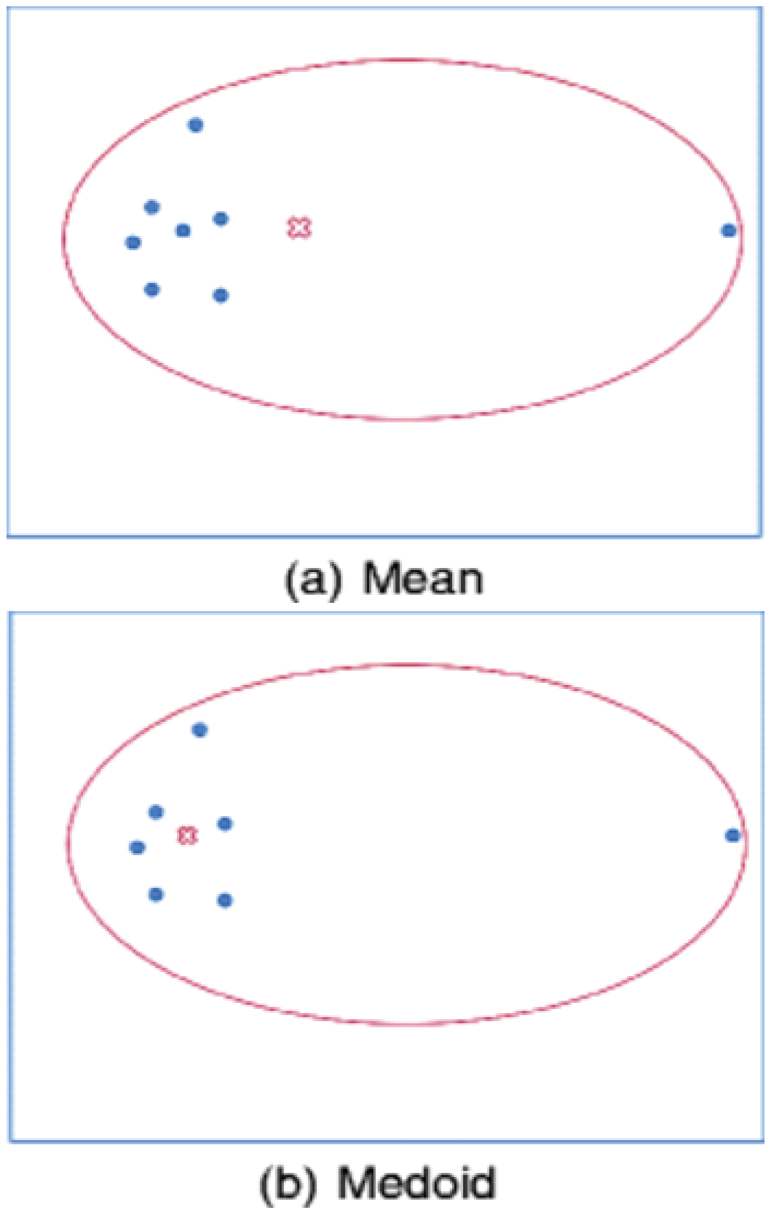
To allow things to be recognized through the process of assembling sensory information into a useful and reliable representation of the world, there are many methods available for feature binding and sensory segmentation in practice. Currently, the most competitive approaches for image segmentation are formulated as clustering models for probabilistic grouping of distributional feature vectors. Clustering is the process of partitioning a set of objects into clusters so that objects within a cluster are similar to each other while objects in different clusters are dissimilar [1]. Over the past two decades, clustering has drawn considerable attention within the data mining research community and as a result, much progress has been realized. Being applied in many important and different fields ranging from statistics, computer science, biology to social sciences or psychology [2-4], it has generated enormous interests, and various techniques have been developed for this purpose in recent years, namely partitioning based approaches, connectivity based approaches (hierarchical clustering), distribution based approaches, density-based approaches, graph-based approaches and recent developments for high dimensional data. Being a partitioning based approach, K-means clustering technique (or sometimes called Lloyd-Forgy method) was developed by James MacQueen in 1967 [5] as a simple centroid-based method and is still one of the most widely used algorithms for clustering [6]. Given a data set, K-means clustering iteratively finds k centroids and assigns every object to the nearest centroid, where the coordinate of each centroid is the mean of the coordinates of the objects in the cluster. It is well known that K-means algorithm is quite efficient in terms of the computational time for large datasets. Unfortunately, it is known to be sensitive to the outliers. For this reason, K-medoids clustering algorithm was proposed where representative objects called medoids are considered instead of centroids [7]. Because it is based on the most centrally located object in a cluster, it is less sensitive to outliers (as illustrated in Figure 1) and the dimensionality of a dataset in comparison with the K-means clustering. The PAM or K- medoids algorithms have been applied to various fields [8-11]. However, despite its many practical applications, K-medoids clustering algorithm suffers from several drawbacks. For one example, it is sensitive to initialization. For another example, it can become trapped in local optima. Finally and most importantly, it works inefficiently for large data sets due to its time complexity [1]. To improve, Kaufman and Rousseeuw (1990) also proposed an algorithm called CLARA (Clustering Large Applications), which applies the PAM to sampled objects instead of all objects. Instead of finding medoids for the entire data set, CLARA considers a small sample of the data with fixed size (sampsize) and applies the PAM algorithm to generate an optimal set of medoids for the sample. The quality of resulting medoids is measured by the average dissimilarity between every object in the entire data set and the medoid of its cluster, defined as the cost function. CLARA repeats the sampling and clustering processes a pre-specified number of times in order to minimize the sampling bias. The final clustering results correspond to the set of medoids with the minimal cost.

In this paper, we propose an aggregation based K-medoids clustering algorithm, which, when combined with CLARA algorithm, manifests its computational efficiency and competency with state-of-the-art partition-based clustering techniques. Basically, it works by first dividing a dataset into several partitions to each of which K-medoids is applied to decrease computation time, and subsequently integrating the clustering results using CLARA algorithm. The aim of this divide-and-conquer hybridization is to increase the robustness and consistency of the clustering results and to significantly reduce the computation complexity. One important contribution of the proposed method is its enhanced ability to detect potential clusters. Another important contribution of the proposed method is its significant tempo efficiency for large data sets. A third important contribution of the proposed method is its significant spatial efficiency in the sense that our methods only need to temporarily store a small number of data points during the clustering process, and can release them when not needed. This third contribution is an advantage over standard K-medoids clustering methodologies, which requires to hold in main memory all the data points and their pairwise dissimilarity, which is otherwise seldom feasible when memory is limited. Finally, to be as general as possible, our algorithm has no specific requirements on the dimensionality of data sets and explores the application to clustering in large high-dimensional image data sets. A number of experiments have demonstrated the robustness and efficiency of the proposed approach in comparison with several other state-of-the-art clustering algorithms for large image data sets.

The rest of the paper is organized as follows. In the next section, we review some existing work on K-medoids based clustering techniques. We then present our proposed approaches After that, an empirical study is conducted to evaluate the performances of our algorithms with respect to several other state-of-the-art clustering algorithms, i.e., MST-based clustering algorithm [12] and CLARA [13]. Finally, conclusions are made and future work is discussed.

Related Work

K-medoids or Partitioning Around Medoid (PAM) method was proposed by Kaufman and Rousseeuw [7] and is known to be most powerful among many algorithms for K-medoids clustering. However, it works inefficiently for a large data set due to its time complexity [1]. Proposed in 1990 by Kaufman and Rousseeuw as an improvement, CLARA applies the PAM to sampled objects instead of all objects. However, it is reported by Lucasius, et al. [14] that the performance of CLARA drops rapidly below an acceptable level with increasing number of clusters. To improve, Lucasius, et al. proposed a new approach of K-medoid clustering using a genetic algorithm, whose performance is reported as better than CLARA but computational burden increases as the number of clusters increases [14]. In 1994, Ng and Han proposed an efficient PAM-based algorithm, which updates new medoids from some neighboring objects [15]. In 2003, van der Laan, et al. tried to maximize the silhouette proposed by Rousseeuw in 1987 [16] instead of minimizing the sum of distances to the closest medoid in PAM [17,18]. To further reduce the computational time, Zhang and Couloigner proposed to utilize triangular irregular network concept when calculating the total cost of the replacement in swap step of PAM in 2005 [19]. To reduce the sensitivity of PAM to the initial medoids, a simple and fast K-medoids algorithm (hereafter this algorithm will be referred to as the FastK algorithm) was proposed by Park and Jun in 2009 [20]. In this algorithm, the density of each object is calculated first and then the smallest k density values are selected as the initial medoids, which improves the clustering performance. However, the initial medoids optimized by this algorithm usually appear in the same cluster, which reduces the final clustering performance. To address the importance of the number of clusters, the variance enhanced K-medoids clustering algorithm was proposed in 2011 by Lai and Hu [21] and the modified silhouette width plot in conjunction with PAM (mPAM) algorithm was proposed by Ayyala and Lin in 2015 [22], which iteratively increase the number of clusters until the evaluation index value is lower than a given threshold. To prevent the algorithm from becoming trapped in a local optimum, in 2013, Mohammad Razavi Zadegan, et al. introduced a new function that ranks objects according to their similarities and their hostility values so as to select the new updated medoids, which can aid in finding all the Gaussian-shaped clusters [23]. To currently be the best algorithm for both selecting the medoids and determining the number of clusters simultaneously, in 2014, Rodriguez and Laio proposed a new algorithm, the density peaks clustering algorithm, based on two assumptions: (1) that cluster centers are surrounded by neighbors with lower local density and, (2) that cluster centers are relatively far from any points with a higher local density [24]. In order to improve clustering performance, especially clustering accuracy in 2015, Broin, Smith and Golden used the genetic algorithm (GA) to both perform a global search and provide multiple initializations for the K-medoids algorithm, reducing the potential impact of poorly chosen starting medoids [25]. To optimize the initial medoids of the K-medoids clustering algorithm, in 2016, Xie and Qu proposed two more improved K-medoids clustering algorithms, the density peak optimized K-medoids (DPK) algorithm and the density peak optimized K-medoids with new measure (DP-NMK) algorithm. However, both algorithms require a cut-off distance based on density peaks and the number of nearest neighboring objects, which would significantly affect the clustering performance, but for which Xie and Qu did not provide a general solution [26]. More recently in 2018, Yu et al. proposed an improved K-medoids clustering algorithm which preserves the computational efficiency and simplicity of [27] while improving its clustering performance. The proposed algorithm requires determining the candidate medoids subsets and calculating the distance matrix, then using both of them to incrementally increase the number of cluster and new medoids from 2 to k, as well as selecting two initial medoids. Experimental results on both real and artificial data sets show that the proposed algorithm outperforms the other three algorithms. The complexity of this proposed algorithm was analyzed to be lower than DPK and DP-NMK, and be similar to FastK.

To summarize, improving the K-medoids clustering performance and computational efficiency remains the main goal among all the previous approaches, whether one is optimizing the initial medoids selection or optimizing the updating medoids method. However, most of these algorithms are based on PAM, so the computational burden still remains. Further, although different approaches for random sampling are described in [28-34], no approach has been proposed to focus on dividing datasets into small partitions and employ a divide-and-conquer paradigm.

The Proposed Approach

An improved K-medoids algorithm

To be less sensitive to outliers, we put a constraint on the maximum and minimum cluster sizes rather than on the number of clusters. The advantage of this constraint is the avoidance of a few largest clusters and an unnecessary large number of small clusters. Given a dataset to cluster, a loose estimate of minimum and maximum numbers of data items in a cluster can usually be available. And the number of clusters in the dataset can be figure out by this constraint. To be less sensitive to initialization and outliers and to prevent from being trapped in local optima, which are caused by selecting the k medoids randomly and swapping all pairs of medoids and non-medoids, we propose that the initial k medoids should be determined with an additional condition that they are selected such that the sizes of all formed clusters are larger than a loosely estimated lower-bound number of objects. On the other hand, when doing medoids' update, the swapping can only be conducted if no resulted cluster has a number of data objects inside it which is smaller than the lower bound. For the K-medoids clustering algorithm to be efficient, our proposed approach is based on the following two observations. Firstly, better effectiveness in clustering performance can be achieved if a small number of well separated clusters exist in a simple clustering task. Better runtime efficiency can be achieved if K-medoids clustering algorithm is applied to a small number of observations. With data size being reduced, more elaborate K-medoids clustering algorithm can be applied to obtain better results. With all these ideas in mind, a new K-medoids algorithm is developed in the following.

Suppose that n objects having p variables each should be grouped into k (k < n) clusters, where k is assumed to be given. The Euclidean distance is used as a dissimilarity measure in this study although other measures can be adopted. The Euclidean distance between object i and object j is given by,

$$d_{ij}=\sqrt{{\displaystyle \sum _{m\text{ = 1}}^p{\left(x_{im}\text{ - }{x}_{jm}\right)}^2}}i\text{ = 1, }\mathrm{...}\text{, }n\text{; }j\text{ = 1, }\mathrm{...}\text{, }n\text{ (1)}$$

Given a loose estimate of minimum and maximum numbers of data items in a cluster, the proposed algorithm is composed of the following three steps.

Step 1: (Select initial medoids)

1. Calculate the distance between every pair of all objects based on the chosen dissimilarity measure (that is, Euclidean distance in this case).

2. Calculate v_j for object j as follows:

$$v_j\text{ = }{\displaystyle \sum _{i\text{ = 1}}^n\frac{d_{ij}}{{\displaystyle \sum _{l\text{ = 1}}^n{d}_{il}}}},j\text{ = 1, }\mathrm{...}\text{, }n\text{ (2)}$$

3. Sort v_j's in ascending order. Select the object having the smallest value as the first initial medoid. Next, starting from the last object having the largest v_j value, with these two medoids, do a clustering. If both the resulted clusters have a size larger than the lower bound (i.e., the estimated minimum number of objects), select it as the second initial medoid. This process proceeds until k objects are selected as initial medoids such that all the resulted initial clusters each have a size large than the lower bound.

4. Obtain the initial cluster result by assigning each object to the nearest medoid.

5. Calculate the sum of distances from all objects to their medoids.

Step 2: (Update medoids)

1. Find a new medoid of each cluster, which is the object minimizing the total sum of the distances to other objects in its cluster.

2. Update the current medoid in each cluster by replacing with the new medoid only when doing so can result in a clustering that all the resulted clusters each have a size large than the lower bound.

Step 3: (Assign objects to medoids)

1. Assign each object to the nearest medoid and obtain the clustering result.

2. Calculate the sum of distances from all objects to their medoids. If the sum is equal to the previous one, then stop the algorithm. Otherwise, go back to Step 2.

K-medoids clustering for image segmentation

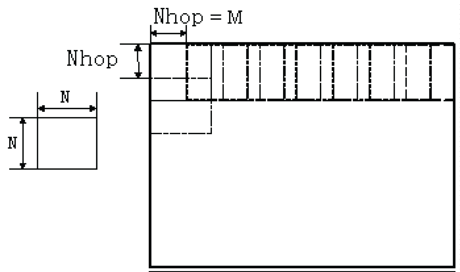
Natural images contain statistical regularities which distinguish objects from each other and from random noise. For successful visual recognition, each object must have attributes that can be used to differentiate it from others and to segment the whole image into meaningful objects. For image segmentation and object identification, instead of using the color information of a single pixel, color pixels in a small local region of an image are considered to form a color histogram-based feature vector. As illustrated in Figure 2, to obtain feature vectors, for a given image, a moving window of size N × N hops by M pixels in the row and column directions but not to exceed the border of the image. The moving windows are overlapping to allow a certain amount of fuzziness to be incorporated so as to obtain a better segmentation performance. The window size controls the spatial locality of the result and the window hopping step controls the resolution of the result. A decrease in the step gives rise to an increased resolution but an increased processing time.

For perceptual grouping, histogram clustering model (HCM) was proposed in [35]. To segment an image using HCM, the image is first decomposed into U not necessarily disjoint image patches, each having W features (or bins). For each image patch $i\in U$, a histogram (h_i,j)1 ≤ j ≤ W is defined as a tuple $h_i\in U^W$. If u_i denotes the number of observations (e.g., pixels) belonging to image patch i, then, u_i = ∑_j h_i,j. The probability to observe features j in a given image patch i can be estimated by

$$p_i\text{ = }{\left(p\left(j|i\right)\right)}_{1\le j\le W}\text{ (3)}$$

where the empirical conditional probability is,

$$p\left(j|i\right)\text{ = }\frac{h_{i,j}}{u_i}\text{ (4)}$$

Based on the feature vectors extracted from image patches, image segmentation can be realized by partitioning the set of image patches into a number of disjoint clusters or segments. By this way, the spatial content organization of image objects has been maintained. Then the segmented images consist of object labels, which results in a much size-reduced learned version of the original ones that can be stored separately and used as indexing files. The model has been successfully applied to image segmentation tasks using feature vectors consisting of high dimensional color histograms and 80 Gabor wavelet texture measures [36,37].

Cluster merging

To apply K-medoids clustering algorithm to data sets too large to fit into the main memory at once, some data preprocessing comes in handy. As introduced in the related work part, CLARA algorithm works on a small randomly selected portion of the whole dataset. Although the algorithm makes it possible for a single machine to K-medoids cluster large data sets more efficiently than K-medoids, it may miss some small clusters existing in a large dataset. That is, after the preprocessing (that is, the sampling) of CLARA, if it happens that the set of randomly selected points does not include all the clusters in the original dataset, some important clusters but of relatively small sizes will be missed. As an improvement, our proposed algorithm is presented in the following for image segmentation task.

Suppose that we are given a sequence of images taken in an unknown environment and our goal is to identify all the objects in the images in terms of patch-based local color features extracted from the images. To fulfill the task, as in the previous subsection, the improved K-medoids clustering algorithm is applied to segment each image, producing a number of clusters for each image. By this way, it is possible that data points belonging to different clusters may be labeled with the same cluster label while data points belonging to one cluster are clustered into different clusters in different images. The next step would be to merge the clusters coming from the same object effectively and efficiently.

Though simple and elegant, K-medoids algorithm in the presence of a large database of object models is not very efficient. To support efficient cluster merging, CLARA algorithm is employed in the current research to reduce the computation cost. Instead of finding medoids for the entire data set, CLARA considers a small sample of the data with fixed size (sampsize) and applies the PAM algorithm to generate an optimal set of medoids for the sample. The quality of resulting medoids is measured by the average dissimilarity between every object in the entire data set and the medoid of its cluster, defined as the cost function. CLARA repeats the sampling and clustering processes a pre-specified number of times in order to minimize the sampling bias. The final clustering results correspond to the set of medoids with the minimal cost. The algorithm runs as follow,

1. Split randomly the data sets in multiple subsets with fixed size (sampsize).

2. Compute PAM algorithm on each subset and choose the corresponding k representative objects (medoids). Assign each observation of the entire data set to the closest medoid.

3. Calculate the mean (or the sum) of the dissimilarities of the observations to their closest medoid. This is used as a measure of the goodness of the clustering.

4. Retain the sub-dataset for which the mean (or sum) is minimal. A further analysis is carried out on the final partition.

Note that, each sub-dataset is forced to contain the medoids obtained from the best sub-dataset until then. Randomly drawn observations are added to this set until sampsize has been reached.

Aiming to reduce the size of the data sets, classical K-means is used in our method as a preprocessor because of its favorable computational properties and the simplicity of the implementation. In this case, the overall CLARA-based cluster-merging algorithm takes the following form: 1) Coarsen the original labeled dataset by using the preprocessor to collapse neighboring data points into a set of local "representative points," 2) run CLARA clustering algorithm on the set of representative points, and 3) assign cluster memberships to the original data points based on those of the representative points.

Algorithm description

With a set of images being the input and a set of segmented images being the output, the overall proposed clustering algorithm runs as follow,

1. The clustering step: Read in an image, extract the feature vectors, apply the improved K-medoids clustering algorithm to segment it and assign a label to each feature vector. This step continues until the end of the image sequence is reached.

2. The merge step: Use the classical K-means algoithm as a preprocessor to reduce the dataset size and apply CLARA to cluster the obtained local "representative points" and merge clusters.

3. Finally, each cluster after integration is marked by a different color, and the results of image segmentation are obtained.

Time complexity analysis

The time complexity of the original K-medoids clustering algorithm is,

$$O_{k-medoids}\text{ = }O\left(k{\left(n-k\right)}^2\right)\text{ (5)}$$

The time complexity of the proposed aggregation based K-medoids clustering algorithm is,

$$O_{overall}\text{ = }O\left(m\left(k{\left(\frac{n}{m}-k\right)}^2\right)\right)+O\left(k^{\text{'}}nt\right)+O\left(k^{\text{'}\text{'}}{s}^2+k^{\text{'}\text{'}}\left(n_c-k^{\text{'}\text{'}}\right)\right)\text{ (6)}$$

where n is the whole data size, m is the number of images, k, k' and k'' are the number of clusters, t is the number of iterations, s is the sampsize, and n_c is the size of local representative points after the preprocessing using K-means algorithm. The first term is the time complexity of the improved K-medoids clustering applied to m images. The second term is the time complexity of the K-means algorithm. The third term is the time complexity of the CLARA algorithm on n_c local representative points. As demonstrated in performance evaluation section, the proposed algorithm can achieve significant speedup with no degradation in clustering accurarcy.

A Performance Study

In this section, we present the results of an experimental study performed to evaluate the proposed aggregation based K-medoids clustering algorithm. First, the clustering performance of the proposed method is evaluated on a set of real images for four color spaces. We exclusively use image data sets because of their visual convenience for the performance evaluation. We next check the effectiveness of the proposed algorithm by performing comparison with CLARA and MST based clustering algorithms. For this comparison, we would like to show that our proposed K-medoids clustering algorithm can outperform the classic CLARA algorithm and the classic MST based clustering algorithm in the classification accuracy. Finally, we will evaluate our algorithm in the execution time which is also compared with those of the CLARA algorithm and the MST-based clustering algorithm to check the technical soundness of this study. The data set is briefly summarized in Table 1.

We implemented all the algorithms in C++. All the experiments were performed on a computer with Intel Core 2 Duo Processor E6550 2.33GHz CPU and 2GB RAM. The operating system running on this computer is Ubuntu Linux. We use the timer utilities defined in the C standard library to report the CPU time. In our evaluation, the total execution time in seconds accounts for all the phases of the proposed K-medoids clustering algorithm, including those spent on the single images, the K-means preprocessing, and the rest. The results show the superiority of our proposed K-medoids algorithm over the other algorithms.

Image segmentation in four color spaces

Outdoor environments are less structured. In this set of experiments, we exclusively choose images taken from out-door scenes. Our dataset, Data, consists of 8 picutres from the Berkeley Data Set 500 [38]. To accurately express the image content, each of the images is divided into smaller blocks for which RGB color histograms (as described in A.1) of dimension 64, HSV color histograms (as described in A.2) of dimension 64, Opponent color histograms (as described in of dimension 64, Opponent color histograms (as described in described in A.4) of dimension 64 are extracted. More specifically, to obtain feature vectors, for each image, a moving window of size N × N is shifted by M pixels in the row and column directions but not to exceed the border of the image. Each color channel is evenly divided into 4 intervals. All the interval combination can generate 64 different color bins for the generation of color histogram for each image patch. Then, all the pixels in the moving window are assigned to the corresponding possibility, and a feature vector (color histogram) is obtained. To summarize, for the set of images, N = 6 and M = 4, resulting totally 75,208 color histogram based feature vectors. Then, the proposed aggretion-based K-medoids algorithm is applied to cluster these RGB, HSV, Opponent, Transformed color histograms.

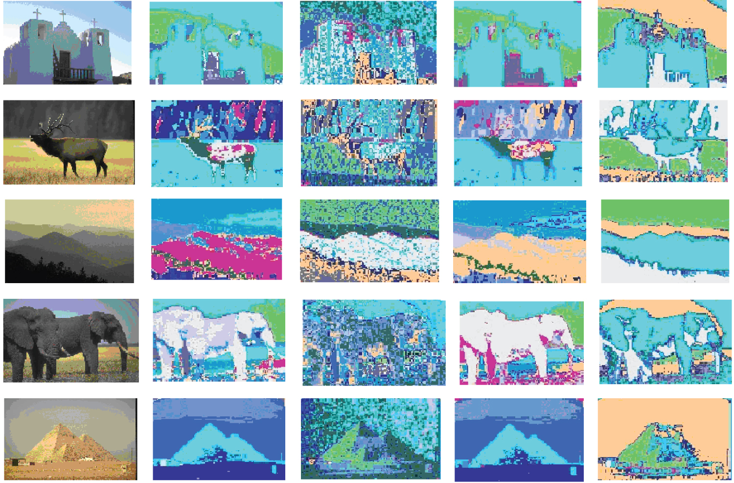
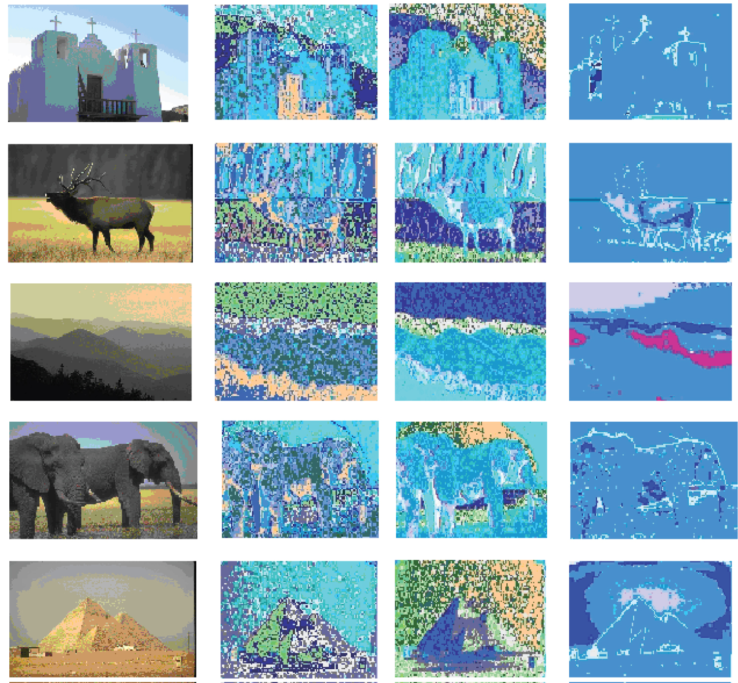
The Berkeley Segmentation Dataset consists of natural images that contain complex layouts of distinct textures, thin and elongated shapes and relatively large illumination changes and is therefore a challenge for segmentation task. Data has 8 different scenes, 5 of which are shown in Figure 3. The first scene is composed of a church building with white wall, three white crosses on the top, a dark brown wood railing entrance in the front, some dark building on the lower-right corner. The second scene is composed of a deer standing on brown to yellowish green grass with a dark green forest behind. The third scene has several undulating mountains in different colors under a setting sun. The fourth scene has two elephants with the left one's head being occluded by the right one's body. The last scene contains a golden pyramid on a desert in front of a light grayish sky. There are five columns in this figure. The first column of Figure 3 displays the five testing images used. The second column of Figure 3 displays the clustering results of our proposed method for HSV color histograms. The third column of Figure 3 displays the clustering results of our proposed method for Opponent color histograms. The fourth column of Figure 3 displays the clustering results of our proposed method for RGB color histograms. Finally, the last column of Figure 3 displays the clustering results of our proposed method for Transformed color histograms. To display results, in the segmented images, four close but slightly different sets of colors are used to denote the percepts.

There are 17 clusters obtained from this dataset by our method. From the segmented figures, it can be seen that our proposed algorithm performs worst clearly in the Opponent color space while reasonably well in the other three color spaces. In the Transformed color space, our method can separate the sky from the church wall and thus performs the best for the first scene. In the RGB color space, our method performs the best for the fourth scene.

To summarize, overall, our algorithm can discover all the major percepts most of time and discriminate percepts in four color spaces.

Performance comparisons

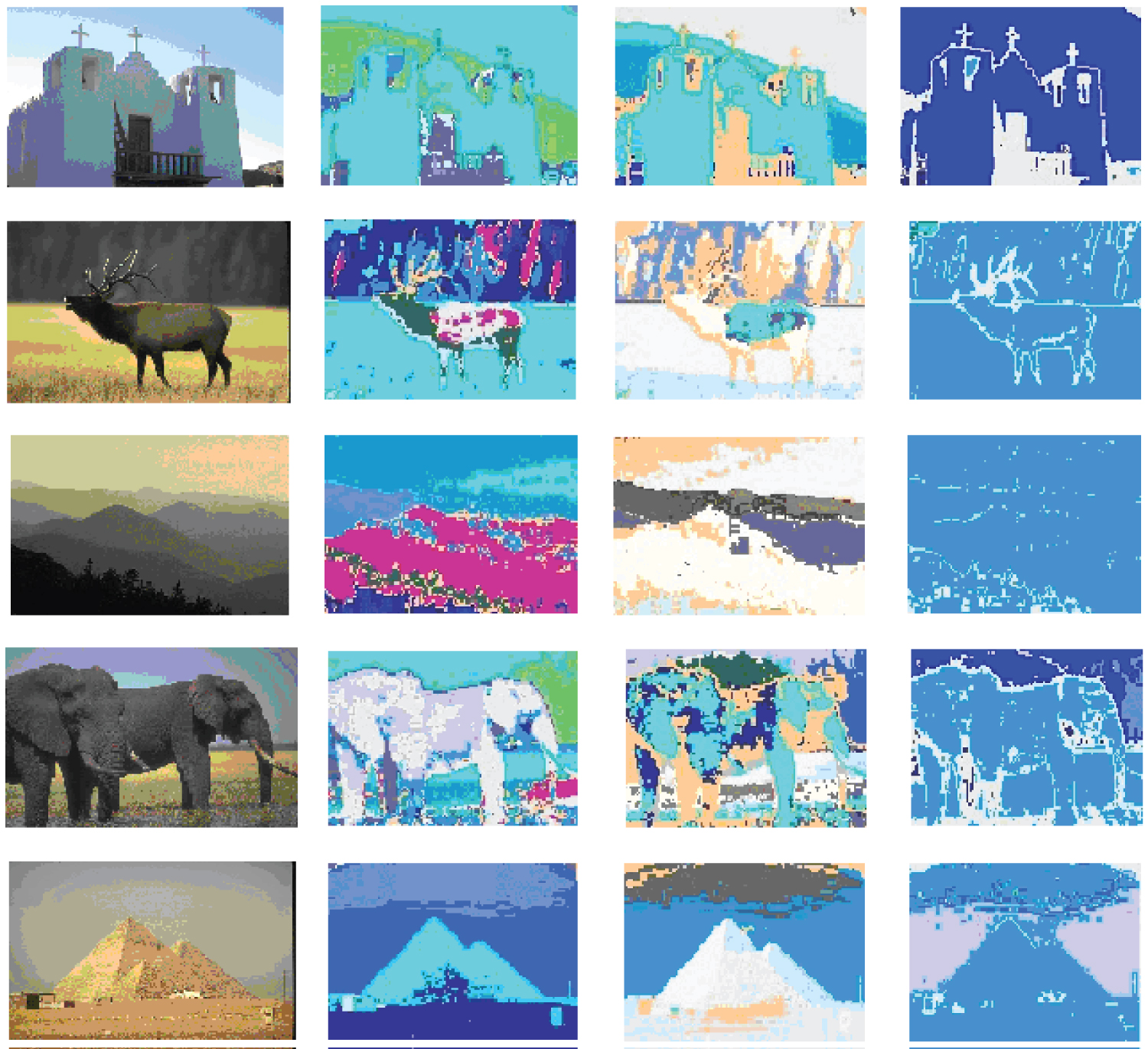
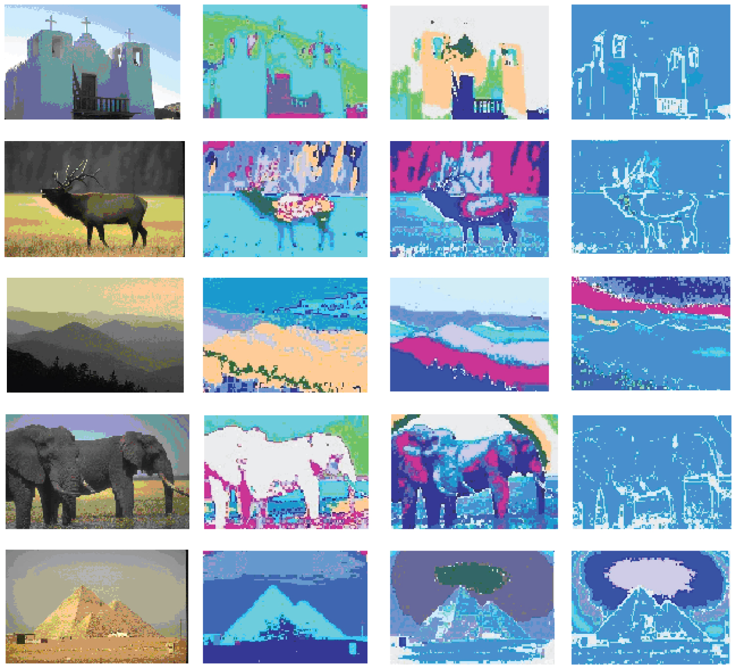
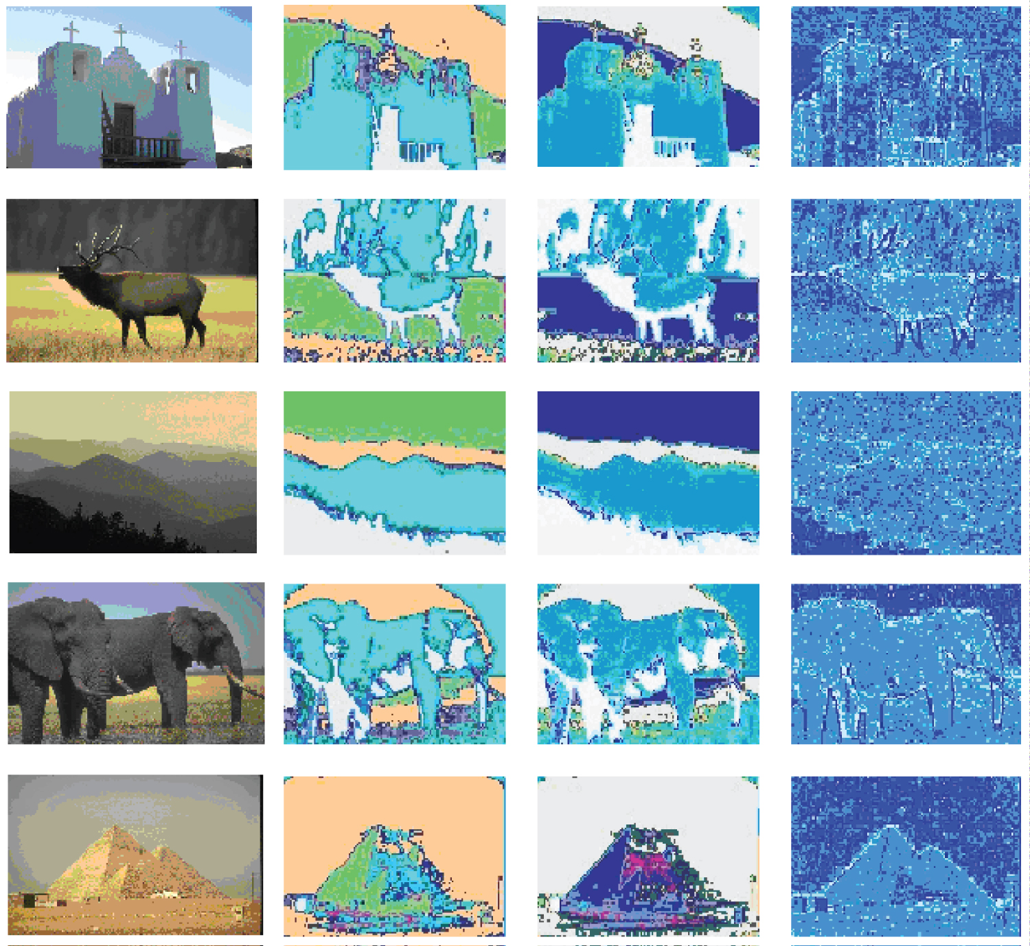
In this set of experiments, three clustering algorithms, our proposed aggretion-based K-medoids algorithm, CLARA clustering algorithm and MST-based clustering algorithm, are applied to the HSV, Opponent, RGB and Transformed color histograms for the image data, Data. Since MST-based clustering algorithm is well known to be good at detecting clusters with irregular boundaries, the performance of our proposed algorithm is compared with that of its. The results are presented in Figure 4 (for HSV color space, respectively), Figure 5 (for Opponent color space, respectively), Figure 6 (for RGB color space, respectively), Figure 7 (for Transformed color space, respectively), respectively, for five images from the dataset in order to keep the amount of data presented reasonable, but consistent performance results are obtained for other images. There are four columns in each figure. The pictures shown in the first columns are the original images. The pictures shown in the second columns are the segmented images using our proposed aggregation based method. The pictures shown in the third columns are the segmented images obtained by running the CLARA algorithm on the whole color histogram based feature vectors extracted from the 8 images (i.e., 75,208 for Data). The pictures shown in the fourth columns are segmented images obtained by running the MST-based clustering algorithm on Data. The results show that different methods have different optimal segmenting results in terms of the number of clusters and in different color spaces. There are 17, 21, and 17 clusters obtained for Data using our proposed aggregation based K-medoids, CLARA and MST based clustering algorithm, respectively.

The results of image segmentation in HSV color space are shown in Figure 4. From the segmented images in Figure 4, it can be seen that our proposed method works better than the other two most of the time. For the first scene, CLARA can separate the sky from the church wall and thus performs the best. Our method performs the next but better than MST based method. For the second, the third and the fifth scenes, our method performs the best and CLARA performs the next.

For the fourth scene, our method performs the best and MST based method performs the next. For all the scenes, MST based method is good at detecting the boundaries.

The results of image segmentation in Opponent color space are shown in Figure 5. From the segmented images in the figure, it can be seen that, in this color space, CLARA and our algorihtm perform similarly and better than MST based method for all the scenes.

The results of image segmentation in RGB color space are shown in Figure 6. From the segmented images in Figure 6, it can be seen that our method works the best for the first, the second, the fourth and the last scenes. CLARA performs a little better than ours for the third scene. MST-based method works the worst for the first four scenes but similarly with CLARA for the last scene.

The results of image segmentation in Transformed color space are shown in Figure 7. From the segmented images in Figure 7, it can be seen that, in this color space, our algorihtm outperforms CLARA in the first and fourth scenes, and works similarly with CLARA in the second, the third and the last scenes. MST based method does not do well for all the scenes.

Overall, the results presented above offer good evidence that our method performs very well on a variety of images from different outdoor domains.

Running time performance

The numbers of local representative points as the ouput from the K-means algorithm and input to the CLARA in our aggregation stage are presented in Table 2. The running time performances of our proposed algorithm, CLARA algorithm and MST based clustering algorithm are summarized in Table 3 for Data.

It can be seen from the table that our method and CLARA use a similar amount of time to segment 8 images, which however is significantly shorter than the MST based clustering method. This is because MST based clustering algorithm requires an MST be constructed in the first place and therefore, is time consuming.

Conclusion

We have proposed a fast aggregation-based K-medoids clustering algorithm and applied it to image segmentation tasks. Basically, our algorithm applies the proposed K-medoids algorithm to segment each image in an image sequence and uses CLARA algorithm for cluster merging. The algorithm significantly reduces the expense of the computation in classic K-medoids algorithm, while retaining good control on the clustering accuracy. Evaluation on an image segmentation task shows that a significant speedup for K-medoids clustering can be achieved by our algorithm in comparison to the original K-medoids algorithm and that better clustering accuracy can be obtained by our algorithm with respect to the CLARA algorithm. However, although image segmentation tasks using feature vectors consisting of high dimensional color histograms have been explored in [36,37], in this work, the dimensions of the feature vectors are not very high. In our future work, we will focus on ex- tending the current research to large and high dimensional color histograms.

Appendices

Images and videos taken from a camcorder are stored for each frame as a RGB (red, green, blue) color image.

RGB color histogram

The RGB histogram is a combination of three 1D histograms based on the R, G, and B channels of the RGB color space. This histogram possesses no invariance properties. More specifically, to obtain the color features in RGB color space, the R is evenly divided into r intervals, while the G and the B are evenly divided into s and t intervals, respectively. Thus, each of them is divided into three parts: r R color values, s G color values, and t B color values. All the interval combination can generate r × s × t different color feature dimensions. Then, all the pixels in the moving window are assigned to the corresponding possibility, and a highly sparse feature vector (color histogram) is obtained.

HSV color histogram

The RGB color images are converted to the HSV (Hue Saturation Value) color space for HSV color histogram computation. The Hue describes each color by a normalized number in the range from 0 to 1 starting at red and cycling through yellow, green, cyan, blue, magenta, and back to red. The Saturation describes the vibrancy of the color and represents the purity of a color such as the "redness" of red. The less saturation in a color, the more pale it looks (washed out). The Value describes the brightness of the color. For normalized RGB values in the ranges from 0 to 1, the conversion to HSV is done in the following manner,

$$H\text{ = }\left\{\begin{array}{c}\left(0+\frac{G-B}{MAX-MIN}\right)\times 60ifR\text{ = }MAX\text{,}\\ \left(2+\frac{B-R}{MAX-MIN}\right)\times 60ifG\text{ = }MAX\text{, }\\ \left(4+\frac{R-G}{MAX-MIN}\right)\times 60ifB\text{ = }MAX\text{,}\end{array}\right.\text{ (A-1)}$$

$$S\text{ = }\frac{MAX-MIN}{MAX}\text{ (A-2)}$$

V = MAX    (A-3)

where MAX is the maximum value of (R, G, B), and MIN is the minimum. From the above formulas, it can be seen that, if MAX = MIN, H is undefined and S = 0, there is no hue and the color lies along the central line of grays, and that, if MAX = 0, V = 0 and S is undefined, the color is pure black and there is no hue, saturation and value.

As the outputs of the above formulas, the Hue values range from 0 to 360, and the Saturation and Value values range from 0 to 1. The Hue values are next normalized to be in the range [0.00, 1.00]. Orange with a bit of red lies in the range [0.00, 0.05], yellow lies in the range [0.05, 0.14], yellow-green lies in the range [0.14, 0.22], green lies in the range [0.22, 0.28], blue-green lies in the range [0.28, 0.45], blue lies in the range [0.45, 0.54], blue-violet lies in the range [0.54, 0.75], purple lies in the range [0.75, 0.81], red-violet lies in the range [0.81, 0.92], and red lies in the range [0.92, 1.00]. To extract color features, a histogram of color measurements in the HSV space for each object is computed as follows. The hue is broken into r bins of equal width. The saturations and values are evenly distributed into s and t bins, respectively. Each color can be represented by combining the three bins, one from the hue bins, one from the saturation bins and one from the value bins. All possibilities of the combinations equal r × s × t different feature color bins for the histogram. The histogram can then be constructed for an image patch by looking at each color feature and finding the number of pixels in the patch that correspond to that feature. After doing this for all the color features in the object, there are r × s × t numbers, each representing the number of pixels of a certain color in the selection patch. The total number of pixels in the selection patch divides these r × s × t numbers, resulting in a highly sparse feature vector of a dimension as high as r × s × t.

Opponent color histogram

The opponent histogram is a combination of three 1D histograms based on the channels of the opponent color space,

$$\left(\begin{array}{c}{O}_1\\ O_2\\ O_3\end{array}\right)\text{ = }\left(\begin{array}{c}\frac{R-G}{\sqrt{2}}\\ \frac{R+G-2B}{\sqrt{6}}\\ \frac{R+G+B}{\sqrt{3}}\end{array}\right)\text{ (A-4)}$$

The intensity information is represented by channel O₃ and the color information by O₁ and O₂. Due to the subtraction in O₁ and O₂, the offsets will cancel out if they are equal for all channels (e.g., a white light source). This is verified by substituting the unknown illuminant with offset o₁:

$$\left(\begin{array}{c}{O}_1\\ O_2\end{array}\right)\text{ = }\left(\begin{array}{c}\frac{R^c-G^c}{\sqrt{2}}\\ \frac{R^c+G^c+B^c}{\sqrt{6}}\end{array}\right)\text{ = }\left(\begin{array}{c}\frac{\left(R^u+o_1\right)-\left(G^u+o_1\right)}{\sqrt{2}}\\ \frac{\left(R^u+o_1\right)-\left(G^u+o_1\right)-2\left(B^u+o_1\right)}{\sqrt{6}}\end{array}\right)\text{ = }\left(\begin{array}{c}\frac{R^u-G^u}{\sqrt{2}}\\ \frac{R^u-G^u-2B^u}{\sqrt{6}}\end{array}\right)\text{ (A-5)}$$

Therefore, these O₁ and O₂ are shift-invariant with respect to light intensity. The intensity channel O₃ has no invariance properties.

Transformed color histogram

An RGB histogram is not invariant to changes in lighting conditions. However, by normalizing the pixel value distributions, scale-invariance and shift-invariance is achieved with respect to light intensity. Because each channel is normalized independently, the descriptor is also normalized against changes in light color and arbitrary offsets,

$$\left(\begin{array}{c}{R}^{\text{'}}\\ G^{\text{'}}\\ B^{\text{'}}\end{array}\right)\text{ = }\left(\begin{array}{c}\frac{R-{\mu }_R}{{\sigma }_R}\\ \frac{G-{\mu }_G}{{\sigma }_G}\\ \frac{B-{\mu }_B}{{\sigma }_B}\end{array}\right)\text{ (A-6)}$$

With μ_c the mean and σ_C the standard deviation of the distribution in channel C computed over the area under consideration (e.g., a patch or image). This yields, for every channel, a distribution where μ = 0 and σ = 1.

Acknowledgment

The authors would like to thank the National Science Foundation of China and that of Shaanxi Province for its valuable support of this work under Grant 61473220 and 2020JM046.

References

1. J Han, M Kamber, AKH Tung (2001) Spatial clustering methods in data mining: A survey. In: HJ Miller, J Han, Geographic data mining and knowledge discovery. (edn), Taylor & Francis.
2. J Malik, S Belongie, T Leung, et al. (2001) Contour and texture analysis for image segmentation. International Journal of Computer Vision 43: 7-27.
3. FR Bach, MI Jordan (2004) Blind one-microphone speech separation: A spectral learning approach. Advances in Neural Information Processing Systems 17 (NIPS' 2004), 65-72.
4. Y Weiss (1999) Segmentation using eigen vectors: A unified view. Proceedings of the Seventh IEEE International Conference on Computer Vision, 975-982.
5. JB MacQueen (1967) Some methods for classification and analysis of multivariate observations. 5th Berkeley Symposium on Mathematical Statistics and Probability. University of California Press, 281-297.
6. AK Jain (2008) Data clustering: 50 years beyond Kmeans. In: Daelemans W, Goethals B, Morik K, Machine learning and knowledge discovery in databases. (edn), Lecture Notes in Computer Science, Springer, Berlin, Heidelberg, 5211: 3-4.
7. L Kaufman, PJ Rousseeuw (1987) Clustering by means of medoids. In: Y Dodge, statistical data analysis based on the norm and related methods, North Holland, 405-416.
8. M Arumugam, J Raes, E Pelletier, et al. (2011) Enterotypes of the human gut microbiome. Nature 473: 174-180.
9. Y Ohnishi, W Huber, A Tsumura, et al. (2014) Cell-to-cell expression variability followed by signal reinforcement progressively segregates early mouse lineages. Nat Cell Biol 16: 27-37.
10. D Amorèse, R Bossu, G Mazet-Roux (2015) Automatic clustering of macroseismic intensity data points from internet questionnaires: Efficiency of the partitioning around medoids (PAM). Seismological Research Letters 86: 1171-1177.
11. A Khatami, S Mirghasemi, A Khosravi, et al. (2017) A new PSO-based approach to fire flame detection using K-medoids clustering. Expert Systems with Applications 68: 69-80.
12. O Grygorash, Y Zhou, Z Jorgensen (2006) Minimum spanning tree based clustering algorithms. 2006 18th IEEE International Conference on Tools with Artificial Intelligence (ICTAI'06), 73-81.
13. L Kaufman, PJ Rousseeuw (1990) Finding groups in data: An introduction to cluster analysis. Wiley, New York.
14. B Lucasius, AD Dane, G Kateman (1993) On K-medoid clustering of large data sets with the aid of a genetic algorithm: Background, feasibility and comparison. Analytica Chimica Acta 282: 647-669.
15. R Ng, J Han (1994) Efficient and effective clustering methods for spatial data mining. Proceedings of the 20th international conference on very large databases, Santiago, Chile, 144-155.
16. J Rousseeuw (1987) Silhouettes: A graphical aid to the interpretation and validation of cluster analysis. Journal of Computational and Applied Mathematics 20: 53-65.
17. CP Wei, YH Lee, CM Hsu (2003) Empirical comparison of fast partitioning-based clustering algorithms for large data sets. Expert Systems with Applications 24: 351-363.
18. MJ van der Laan, KS Pollard, J Bryan (2003) A new partitioning around medoids algorithm. Journal of Statistical Computation and Simulation 73: 575-584.
19. Q Zhang, I Couloigner (2005) A new and efficient K-medoid algorithm for spatial clustering. Lecture Notes in Computer Science 3482: 181-189.
20. HS Park, CH Jun (2009) A simple and fast algorithm for K-medoids clustering. Expert Systems with Applications 36: 3336-3341.
21. PS Lai, HC Hu (2011) Variance enhanced K-medoids clustering. Expert Systems with Applications 38: 764-775.
22. D Ayyala, S Lin (2015) GrammR: Graphical representation and modeling of count data with application in metagenomics. Bioinformatics 31: 1648-1654.
23. S Mohammad Razavi Zadegan, M Mirzaie, F Sadoughi (2013) Ranked K-medoids: A fast and accurate rand-based partitioning algorithm for clustering large datasets. Knowledge-Based Systems 39: 133-143.
24. Rodriguez, A Laio (2014) Clustering by fast search and find of density peaks. Science 344: 1492-1496.
25. PÓ Broin, T Smith, A Golden (2015) Alignment-free clustering of transcription factor binding motifs using a genetic-k-medoids approach. BMC Bioinformatics 16.
26. J Xie, Y Qu (2016) K-medoids clustering algorithms with optimized initial seeds by density peaks. Journal of Frontiers of Computer Science and Technology 9: 230-247.
27. Yu D, G Liu, M Guo, et al. (2018) An improve d K-medoids algorithm based on step increasing and optimizing medoids. Expert Systems with Applications 92: 464-473.
28. SS Singh, NC Chauhan (2011) K-means v/s K-medoids: A comparative study. Proc National Conference on Recent Trends in Engineering & Technology.
29. A Patel, P singh (2013) New approach for K-mean and K-medoids algorithm. International Journal of Computer Applications Technology and Research.
30. F Jiang, G Liu, J Du, et al. (2016) Initialization of K-modes clustering using outlier detection techniques. Information Sciences 332: 167-183.
31. T Velmurugan, T Santhanam (2011) A survey of partition based clustering algorithms in data mining: An experimental approach. Inf Technol J 10: 478-484.
32. S Shah, M Singh (2012) Comparison of a time efficient modified k-mean algorithm with K-mean and K-medoid algorithm. 2012 International Conference on Communication Systems and Network Technologies.
33. Q Li, X Liu (2014) A K-medoids clustering algorithm with initial centers optimized by a P system. International Conference on Human Centered Computing, 488-500.
34. M Sood, S Bansal (2013) K-medoids clustering technique using bat algorithm. International Journal of Applied Information Systems 5: 20-22.
35. FCN Pereira, N Tishby, L Lee (1993) Distributional clustering of english words. 31st Meeting of the Association for Computational Linguistics, 183-190.
36. X Wang, M Tugcu, JE Hunter, et al. (2009) Exploration of configural representation in landmark learning using working memory toolkit. Pattern Recognition Letters 30: 66-79.
37. JE Hunter, M Tugcu, X Wang, et al. (2011) Exploiting sparse representations in very high-dimensional feature spaces obtained from patch based processing. Machine Vision and Applications 22: 449-460.
38. R Unnikrishnan, C Pantofaru, M Hebert (2007) Toward objective evaluation of image segmentation algorithms. IEEE Transactions on Pattern Analysis and Machine Intelligence 29: 929-944.