How Droughts Influence Earthquakes

Abstract

Earthquakes result from strain build-up from without and weakening from within faults. A generic co-seismic condition is presented that includes just three angles representing, respectively, fault geometry, fault strength, and the ratio of fault coupling to lithostatic loading. Correspondingly, gravity fluctuations, bridging effects, and granular material production/distribution form an earthquake triad. As a dynamic constituent of the gravity field, groundwater fluctuation is the nexus between the triad components. It is pivotal in regulating major seismic irregularity, by reducing natural (dry, or purely tectonic, stationary seismicity) inter-seismic periods and by lowering magnitudes. Specifically, to exert stress on the fault, groundwater does not need to reside deep in proximity to the locked fault interface, as it can work remotely. It can act mechanically-direct (MD), by a differential de-loading and superimposing a seismogenetic lateral stress field, thereby aiding plate-coupling, from without, or mechanically-indirect (MI) by enhancing fault fatigue, and hence weakening the fault, from within. To verify this hypothesis, gravity measurements, and a numerical model, are used. The remote action hypothesis is globally applicable. Detailed results are presented for the Himalayan and New Zealand regions. The gravity recovery and Climate experiment (GRACE measurements) reveals that major earthquakes (Mw 5 and above) always occur in the dry stage, indicating drought and associated groundwater extraction is an important trigger for major earthquakes. By exploring 73 historical records successfully reproduced by the model, it is found that for collisional (e.g., the peri-Tibetan Plateau) and strike-slip (e.g., the San Andreas Fault) systems, the MD mechanism dominates, because the orographically induced spatially highly variable precipitation is channeled into greater depth by through-cut faults. Droughts elsewhere also are seismogenetic, but likely through MI effects. In a warming future climate, mechanisms identified here play a greater role in increasing the recurrence frequency of major earthquakes, but also in slightly reducing their severity.

Keywords

Tectonic earthquakes, GRACE, Groundwater fluctuations, Bridging effects, Granular material production

Significance Statement

This study formulates co-seismic conditions involving three specific angles that relate to balancing of the magnitude and direction of the associated forces that collectively when perturbed can precipitate an earthquake event. The hypothesis developed in this research (1) Enlarges our knowledge base by extending the canonical frictional phenomena into fatigue conditions at the plate interface; 2) Indicates that large scale, extended droughts, by exerting cyclical unloading, create two mechanisms for enhancing tectonic instability and the associated triggering earthquakes; and (3) Integrates the role of (generic) groundwater fluctuations at the nexus thereby linking climate change caused extremes and perturbations of the tectonic earthquake cycle. With this hypothesis, mechanics-based process modelling has the potential to be used to determine the locations and development of the evolving regional stresses and to answer the questions of why, when and how extreme will be a specific earthquake event.

Introduction

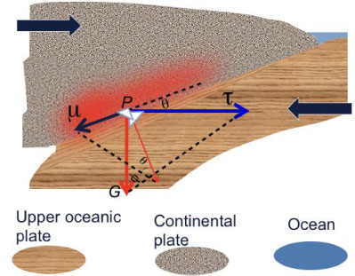
With enhanced hydrological cycles, severe droughts and extreme floods are becoming more frequent. In addition to their direct socio-economic consequences, they also influence seismic activity. There are salient remote sensing signatures from droughts and floods. Relying on the groundwater fluctuation signals provided by gravity satellites, this study focused on revealing the intrinsic link between large scale hydrological cycles and tectonic earthquakes, especially the role of groundwater, and water residing in the rhizosphere, in affecting seismic activity. Tectonic earthquakes are frictional phenomena between plates in contact [1]. At the wedge junction, the upper plate's weight (or more generally, the compressive stress) aids friction in resisting the increasing plate-coupling stress $\text{(}\tau )$ resulting from differential plate motion. Figure 1 is an idealized configuration of uniform fault zone geometry, which assumes a constant slope angle, $\theta$, unlimited width in the transverse direction, and uniform material with a constant maximal frictional coefficient ${\mu }^{\text{'}}=\text{ tan (}{\theta }_f)$. In this cases, the co-seismic condition is:

$${\varphi }_c=\theta \text{ + }{\theta }_f\text{ (1)}$$

where the repose angle is $\varphi \text{ = arctan(}\tau \text{/G)}$, and G is the compressive stress on the shear (fault) zone. The subscript 'c' means the critical value, $\theta$ is the slope of the fault zone, determined by the geometry of the plate interface, and ${\theta }_f$ is the maximum static friction angle corresponding to fault strength. Values of ${\theta }_f$ depend on wall rock material properties and lithology [2,3]. Between seismic events, the repose angle increases steadily and approaches the sum of the fault slope angle and the maximum static friction angle. The driving stress increases and the overall resistive stress decreases (i.e., ${\theta }_f$ decreases); both are seismogenetic [1]. In reality, erosion from within and the loading from without likely are simultaneous. Earthquake cycles are stress adjustment cycles. Closely related to the three angles in Eq. (1) are the earthquake triads: i.e., weight fluctuations of the overriding crust, bridging effects, and fatigue [4]. With the fault strength set as constant, the fault geometry and plate-coupling stress determine a natural, limiting, earthquake occurrence frequency [5]. However, the observed earthquake occurrence seldom obeys this limit and typically occurs well ahead of schedule, due to various fault-weakening factors. Among many other first order mechanisms explainable by Eq. (1), the present study singles out the weight loss (i.e. de-loading) of the upper crust as seismogenetic. As recently reported, for the central Californian valley [6] the weight loss of the upper crust can result from extended droughts that deplete the soil moisture content residing in the rhizosphere and/or by groundwater loss (extraction). By synthesizing geodetic dislocations, obtained from radar and GPS measurements of surface deformation, using an elastic dislocation model, Gonzalez, et al. [7] found that the areas of fault slip, along the Alhambra de Murcia Fault of southeast Spain, correlated well with positive Coulomb stress changes induced by groundwater extraction from nearby aquifers. Water table decreases of hundreds of meters were detected. Thus, the nucleation and main rupture of the Mw 5.1 Lorca earthquake (May 11, 2011) were assumed to be attributable to a loss of groundwater. In the following discussion, groundwater is used as a generic term for both soil moisture, and for drainage into a groundwater reservoir. For relatively weak faults (e.g. subduction megathrusts), the lateral stresses exerted by groundwater extraction are of the same order of magnitude as the fault strength. The normal stress component exerted by groundwater transfers readily into lateral stress in the fault environment. The following discussions use subduction faults and collisional systems with thrust faults as prototypes. By substituting compressive stress for lithostatic loading, the same reasoning also applies to strike-slip faults, as explained in the Supplementary Material of Ref. [6].

Displacements caused by a major earthquake (Mw of 5 or greater) usually range between 0.5-3 m, i.e., they are at least 3 orders of magnitude smaller than the dimension of the seismically locked fault zone, which can be several hundred kilometers. Consequently, material in the locked fault zone has experienced numerous such wearing and tearing events. When simulating near-future earthquakes, the geological backgrounds, including topography, material properties and fault geometry, can reasonably be assumed to be constant. Thus, the natural limiting frequency of seismic slip/rupture occurrence of a fault is highly stable. The irregularity in earthquake occurrence is primarily due to fault weakening mechanisms and to external forcing from the upper boundary. This study focuses on more dynamic fluctuations affecting the earthquake triad. In the Supplementary Material of this study (SM), a stability index is introduced, based on Eq. (1) to explain, simply, the interaction of the triads and the role played by groundwater fluctuations.

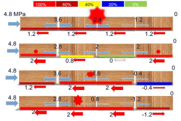
As an under-determined problem, multi-solutions (i.e., uncertainties in the causal mechanisms) in seismogenesis can result from insufficient information about the lateral interactions among different segments of the overriding crust (Figure 2). Rather than the self-weight, the groundwater is influential as it affects the lateral interaction between crust segments. In Figure 2, the upper (usually continental) crust is represented as four "carriages" of a train, each carriage signifying different segments of the upper crust, which is in force balance between the frictional force at the bottom and the drag in the front and therefore it is stationary. Depending on how each carriage is footed (analogous to the friction between the upper and lower crust plates), there are several possible configurations/scenarios (the four rows in Figure 2). If the elastic plate can maintain rigidity over the entire shear zone, all segments of the shear zone must reach stress saturation for coherent sliding to occur. Prior to that critical moment, all segments 'saturate' at the same rate, as the compressive driving stress increases (the top train in Figure 2). In reality, earthquakes involving the 'saturation' of the entire shear zone seldom occur, because tectonic plates have difficulty in maintaining rigidity over extended distances, manifested as the existence of through-cut faults, heave bumps and many small magnitude earthquakes within close proximity of each other. Consequently, many locations do not contribute their shares of resistance and rely on neighbors to stay in place. Depending on how is distributed on the fault zone, there are various possible combinations of saturated and partially saturated segments along the fault zone (trains 2-4 in Figure 2). In Figure 2 it is assumed the distance that plate maintains its rigidity also is the horizontal dimension of each segment. Thus, once saturated, a corresponding co-located earthquake can occur. For example, in the second train (second row of the scenarios) the first and the last segment are saturated. As they are separated, two small magnitude earthquakes (or one event with two small ruptures [8]) are generated. The third train has two adjacent segments saturated. In this case, a larger magnitude earthquake is triggered. The fourth train is unique in that it involves interlaced compression and dilation among the segments, corresponding to a saddle-shaped strain distribution. Consequently, the three adjacent segments are simultaneously saturated and a super earthquake is formed.

Even in the case of this highly idealized fault, with its uniform maximum friction coefficients and uniform lithostatic loading, very different spatial patterns are possible, fostering earthquakes of drastically different magnitudes and at different spatial locations. These examples represent only a fraction of the myriad possibilities that can unfold in reality. In particular, earthquake occurrence can be compounded by any factors that affect $\tau$, G, and ${\theta }_f$ (or fault strength µ') in Eq. (A1). Multi-solutions in seismogenesis result largely from inadequate information as constraints on, or under- determination of lateral interactions. For example, historical data should be treated with caution when predicting future earthquake scenarios because they usually do not provide information on the rupture length, width and slip; they provide essentially no indication of the horizontal coherence of the different plate segments. Earthquakes, because of the relative motion of plates involved, inevitably have footprints on the mass [9,10], energy [11] and momentum fields (Ref. [12] and references therein). Hence, earthquake predictions are increasingly based on observations of these physical parameters and their fields. The mechanism discussed here, i.e. the seismic consequences of groundwater fluctuations, fits this situation exactly. It is a hitherto largely neglected factor that plays a far larger role than anticipated in the existing approaches, which include only local weight effects as some extra weight (negligible compared with the ~20 km thick overriding crust plate). The effect of the groundwater fluctuations is magnified by the bridging effects and the related granular material (GM) generation, which is a fatigue for brittle material.

Groundwater fluctuation caused fatigue accumulated temporally because there is no healing mechanism for the granular fatigue and each leaves an accumulative memory on the plate interface. Unlike the reported good correspondence between minor seismic activity on the San Andreas fault and the central California droughts and groundwater depletion [6], there seems to be no one-to-one correspondence between extreme precipitation and drought cycles and the large earthquakes. It is a multiple drought-wet cycles preceding one major earthquake phenomenon. More critically, the footprint in the lateral stress field accumulates spatially, especially along the frontier mountain chains that act as waveguides by maintaining plate segments' rigidity for extended distances. As it is a grand challenge, it is not surprising that there is no simple equation available that predicts earthquakes. All expressions and equations here are intended to convey the concepts of the earthquake triads. A sophisticated numerical modeling approach, as elaborated in the next section, is needed for reliable seismic hazards predictions.

Materials and Methods

The SM outlines the interactions of the earthquake triads in the simplest possible manner. From Eq. (A1), the weight of the overriding plate always serves as a stabilizing factor. A weight reduction (e.g., from extended droughts) contributes to instability as it is seismogenetic. Fluctuations in the weight of the overlaying plate not only have local stability consequences, they also affect neighboring regions through the bridging effect and a unique fatigue process of the fault zone [13,14], by GM generation and transportation, a common fault-weakening mechanism. Two objects, when pressed against each other, wear and tear at the interface, as a manifestation of material fatigue. The interfaces of tectonic plates are no exception. Production of granular debris is the primary form of fault interface fatigue. Regions of strong contact, likely as a result of the bridging effect, enhance active granular material generation. GM has a much smaller viscosity and acts as a lubricant for the plates involved. Regions carrying more loading now effectively rest on a 'slippery floor' (i.e., more weight is loaded on smooth contacts and less is loaded on rough contacts, along the shear zone). Thus, the bridging effect, by affecting granular material generation and redistribution, influences the frictional properties of the fault interface. It therefore achieves a negative spatial covariance between loading and fault strengths, thereby being seismogenetic according to Eq. (A1). Sources of bridging effects are numerous. For example, large scale structures in the overriding plate, such as mountains and valleys, signify bridging effects at depth on the seismogenetic fault zone [15]. Bridging effects from static geological backgrounds, although they may cause variations in the frictional properties of the seismogenetic zone, change only slowly and are not responsible for short-term variations in major earthquake occurrence. Large scale variations in groundwater, however, are more dynamic and thus are viable candidates for explaining earthquake occurrence irregularity on decadal to centennial time scales. Cyclic forcing is the most effective means of causing fatigue [16]. Cyclic groundwater fluctuations, especially when acting in concord with the resonance frequency of the plates, assist GM generation.

Groundwater time series within and outside the gravity satellite measurements period

Fluctuations in groundwater, which are remotely sensed by gravity satellites such as the Gravity recovery and Climate experiment (GRACE) [17-19] are used to highlight the strong correlations with the timing of major earthquakes. Launched in 2002, GRACE has revolutionized the detection of large- scale mass changes on Earth.

Water changes, irrespective of whether they result from accelerated ice sheet melt, extreme precipitation events, or extended droughts, are the dominant drivers of regional mass fluctuations. In addition to measurement noise, the global monthly one-degree data used in this study have the following missing months: June and July of 2002, June 2011, May and October of 2012, March, August and September of 2013, February and November of 2014, and June 2015. Missing values are obtained by linearly interpolated from neighboring months. In total, there are 15 years of GRACE measurements of time variations in gravity changes over the globe, before the quality of the data degrades. Before 2002, or for areas with land surface areas that are too small to be resolved by GRACE data, a land surface scheme within a model referred to as Scalable Extensible Geofluid Modeling framework for ENvironmenTal issues (SEGMENT [14,20,21], will be detailed in Subsection 2.2), driven by atmospheric parameters, is used to simulate groundwater fluctuations. The earthquake triad is interlinked with groundwater fluctuations. Groundwater-aided GM generation is the mechanism modulating earthquake cycles. As an initial attempt at supporting this hypothesis, global evidence is provided of the earthquake events and gravity fluctuations in the neighboring regions. The present study uses the global seismic records from the USGS Significant Earthquakes Archive (https://earthquakes.usgs.gov).

From Eqs. (1) and (A1), groundwater, by affecting the gravity field, contributes to fault instability. Its spatial fluctuation, through enhancing GM generation, also weakens the fault from within (Section 2.2 of the SM). To obtain the groundwater fluctuations over the past years from 2000-2015, a continuous time marching of the land surface scheme is performed with a 30-minute time step. Atmospheric parameters such as near surface air temperature, humidity, pressure, winds, and radiative components are from the NCEP/NCAR reanalysis. Precipitation data from the Global historical climatology network (GHCN, 1900-2015), GPCP, and The tropical rainfall measuring mission (TRMM, 1998-2015) are taken as inputs during the observational periods to drive the land surface scheme in SEGMENT to diagnose how much precipitation is percolated into ground water reservoir. For the recent decade (2002 onward), GRACE measurements provide a reliable means for the groundwater recharge/discharge. Model simulations are found to be satisfactory when verified against GRACE measurements. GRACE has a very coarse resolution and SEGMENT can provide the spatial distribution of groundwater at much finer resolution. Obtaining groundwater distribution in a warmer climate is challenging. A small ensemble of 27 climate models, listed in Table S1, and an innovative approach in estimating extreme precipitation [20] is used for the prediction of the future occurrence of earthquakes. The partitioning into surface runoff, evapotranspiration and ground water percolation also is performed within SEGMENT.

In addition to the geodetic measurements and atmospheric parameters, the earthquake model used here also requires some static data, such as fault geometry, material property and thermodynamic parameters of the entire simulation domain. In summary, CRUST1.0 [22] is used to set up the geometry and physical properties (e.g., density values) over the grids within the crust layer. It refers to the Advanced Solver for Problems in Earth's ConvecTion (ASPECT) [23] for setting up the thermal and initial flow fields. Model spin up runs are constrained by present GPS measurements of the surface elastic deformation.

Numerical earthquake model

Like landslides, tectonic earthquakes are frictional phenomena. However, the prediction of earthquakes is, however, very challenging and cannot be summarized in just one or a few simple equations. Formulae are used here to explain only the physics involved. At present, the only viable approach is a coordinated solving of a numerical modeling system that includes energy, momentum, and mass conservation principles, under prescribed rheological properties. SEGMENT is such a realization. The current rubric on earthquake prediction and forecasting (e.g., Ref. [24]) comprises four steps: The fault model provides physical geometry of the faults (especially large and active ones) considered; the deformation model provides slip-rate and creep estimates for each fault section, and derives the deformation rate of the modelled faults; the earthquake rate model provides long-term rate of all earthquakes throughout the region of interest; and, finally, an earthquake probability model provides the actual earthquake prediction. SEGMENT essentially covers the first three models (with the fault physical geometry and mechanical parameters as inputs to the modeling system). There is no application of probabilistic methods in earthquake forecasting and the epistemic uncertainties are assumed to be model uncertainty (e.g., model parameter setting and input data inaccuracies), which reflect the still incomplete understanding of earthquake mechanisms. In actual predictions, SEGMENT modeling is a set of parallel code and requires super computers for execution.

An understanding of the basic earthquake mechanics presented here is based on numerical simulations from SEGMENT. SEGMENT is applied as a global spherical crown model, with the stress decomposed into driving stress and resistive stress components, following Van der Veen and Whillans [25]. By solving the equations for conservation of mass, momentum and energy, SEGMENT provides a 3D distribution of strain, stress, and the three components of velocity in the simulation domain. Identifying a major earthquake from these prognostics is described in Section 2.3. In addition to numerical details such as fault-following grid stencils, Section 2.3 also describes approaches in obtaining the current global distribution of GM thickness and its future evolution.

Numerical model setup and parameterization of the earthquake triads

The theoretical concepts/hypothesis discussed above and also in the SM, namely, GM generation facilitated by groundwater fluctuation, is implemented in a global spherical crown model SEGMENT. As a dynamic model unlike kinematic and empirical statistical models, SEGMENT solves the equations of mass, momentum (under assumed multiple rheology), and energy conservation in 3D spherical geometry. The model prognostic equations include the three components of velocity; temperature; and six components of the deviatoric stresses. Their evolution is depicted by forward time marching of the governing equations. Variables in Eqs. (1) and (A1), such as the degree of stress saturation, are diagnostic equations of SEGMENT rather than prognostic equations. Through these diagnostics, the stress build-up during the inter-seismic stage can be followed. A major earthquake in the model is identified from the predicted motion velocities. Once an event is identified, the released energy is estimated within a time window that covers fully the time period with macroscopic slip. An epicenter is diagnosed as the geological locations of the saturated grids, weighted by the respective energy release. The degree of stress saturation S is not directly used to identify earthquakes, because the grid elements are not isolated; there are interactions among adjacent grids. If the unlocking/rupture at a grid point releases large amount of energy, a neighboring grid point, even if distant from (stress) saturation, can be unlocked and set into motion. In fact, some very large earthquakes are formed because there are some sections of the fault (not necessarily adjacent) are simultaneously ruptured and the released energy triggered neighboring sections, resulting in an upward spiral that causes a domino effect in propagating away of the rupture region.

Grid stencil of SEGMENT: For this study, the original 3D spherical model of the upper ~4 km medium (suffices for ice sheets and landslides applications) is now applied to the 500 km thick lithospheric material (including elastic crust and visco-elastic upper mantle). The horizontal resolution is generally 30 km at the Earth's surface and refined to 2 km at the subduction zones (Figure S1). The vertical resolution varies using 101 stretched vertical layers to represent the 500 km depth. A stretching scheme is used so that the shear zone gets higher resolution and is better represented. In setting up the model grids in the simulation domain, it is ensured that there always is a vertical level that has a surface parallel to the oceanic plate's upper surface. That is, SEGMENT uses a fault zone-oriented coordinate system.

Static geological parameters and viscosity parameterizations: The SEGMENT had been used satisfactorily for landslide research in the past. As frictional phenomena, landslides and tectonic earthquakes share high degree of similarity. Both involve a shear zone and weakening of the shear zone leads to instability. Reducing the weight of the overlying portion also is prone to instability for landslides. For example, around manmade reservoirs formed by occluding a river branch with a dam, landslides along the banks always occur during the discharge stage of the reservoir, same de-loading mechanism as presented in Eq. (1) for earthquakes. Although the similarity between landslides and tectonic earthquakes makes the conversion of SEGMENT into an earthquake model feasible, the pressure and thermal environments of the fault interface and the shear zone of landslides are very different. Special attention to the viscosity parameterization is required. Also, direct verification of the schemes become difficult for earthquake applications as the plate interface is deep-buried that direct measurements of either stresses or dislocations are rarely available. Inverse methods are necessary for model verification, spin-up and initialization.

The CRUST1.0 module is used to set up the density values over the grids within the crust layer (both the oceanic and continental crusts). Underneath the bottom of the crust layer is assumed to be upper mantle material (silicates), and is given a uniform reference viscosity of $n_0=\nu {\text{ = 10}}^{\text{19}}Pa•s$ and a density of 3.3 × 103 kg/m³. In setting up the grids above present sea level, the Advanced space- borne thermal emission and reflection radiometer (ASTER) global digital elevation map (asterweb.jpl.nasa.gov/) and ETOPO1 (downloadable from https://www.ngdc.noaa.gov/mgg/global/global.html) bathymetry are referenced to. For faults with intensive gravity measurements, for example the Longmenshan Fault Zone (LFZ, 102-106ºE; 30-33ºN) of the eastern margin of the Tibetan Plateau, there was a detailed gravity survey after the Mw 7.9 Wenchuan earthquake on 12 May 2008. Finer resolution data on elastic plate thickness, density and rigidity profiles are available and used in replacement of the CRUST1.0-derived parameters. Similarly, the Andes survey [26] (and data pointed out by references therein) also provided information that is merged into the coarse resolution CRUST 1.0.

Based on the fact that the co-seismic ruptures consume only a portion of the plate interface [27] to the center and the down-dip section creeps, the upper and lower portions of the plate should be treated respectively as elastic and visco-elastic material. Grids in the upper crust are considered elastic and elastic moduli are specified using canonical values. Grids in the lower crust and upper mantle away from the shear zone are considered to be viscoelastic [12] but becoming more rigid upwards intending a smooth transition in the vertical domain. This is achieved by considering the thermal structure [11] in the parameterization of material viscosity $n(T,P)=n_{0}D\exp [(Q+PV)/\text{R / T]}$. Here P is confining pressure, T is absolute temperature, and D depends on the rock composition, grain size and fluid content. Here Arrhenius' activation energy Q (~75-260 kJ/mol for natural rocks), specific volume V and universal gas constant R (8.314 J/mol/K) all are assumed to be constants in the model. In response to different stress conditions, wall rocks can be compressed or stretched within a narrow range before onset of brittle fatigue. Arrays are allocated to record the amount of granular material formed at each grid cube. The shear zone is a granular zone of variable thickness (Figure S2). In most cases, it is only a small fraction of the shear zone layer that is granular material (also recorded in arrays). The parameterization of GM viscosity follows Ref. [13] as implemented in SEGMENT [14]. The shear-thinning viscosity structure (Eq. 8 in Ref. [14]) implies a shear-localizing effect from GM accumulation. The present amount of GM (Figure S2c) is deduced from surface velocity using the method in Ref. [21]. Future variations of GM are diagnosed (relevant equation is detailed in the next subsection on GM generation that immediately follows). The granular ensemble size is deduced from its parent rock type and the associated grain sizes. Re-mapping of the grid stencils is automatically performed only if the accumulated GM exceeds 20 m or the earthquake caused displacement is greater than 20 m.

The lower boundary stress conditions are critical for the simulation of stress build up inside the simulation domain. The GPS measurements of plate motion speeds $\overrightarrow{V}$ are used to fine tune the parameters of upper mantle layers so that lateral stress (basal drag) exerted on the lowest model layer at the active zones (mantle driven plate motion) and passive zones (plate driven mantle motion) nearly balance. From the vertical profile of the horizontal velocity components it is clear that, for most regions, the mantle motion is passively forced by the overlain plates and only in the active thermal hot spots (for Cascadia, it is the Yellowstone area), does the boundary layer flow structure indicate that it is the mantle flow that exerts a strong drag to the overlain plate. Reflected in the flow structure, mantle flow speeds increase away from the lithosphere-asthenosphere boundary (LAB) rather than being a maximum at the LAB. Therefore, the driving stress is primarily from lateral stress from neighboring grids within the lithosphere, rather than from the local basal drag from mantle (ultimately it is from the convective mantle but local to subduction zones it is not). The upper boundary condition is assumed to be stress-free (i.e., $\tau .\overrightarrow{n}=\text{ 0}$ at upper surface). The model spin-up from ad hoc initial conditions is aided by advanced data assimilation schemes using the remotely sensed plate motion, (weather signal pre-filtered) gravity signal and thermal flux measurements available.

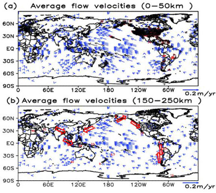
Accurate flow fields are critical for accurate estimations of the stress build-up between plates. Figure 3 shows present plate motion velocities at two vertical levels: 0-50 km and 100-250 km depth averages. The geodetic data over land mass in panel (a) were not collected simultaneously (actually over 1991-2003) but spanned a period of many major earthquakes (e.g., the Mw 6.7 Northridge earthquake). Because major earthquakes during the time window of geodetic data collection may leave coseismic and postseismic effects on the data [28], comparisons between modeled neotectonics and GPS measurements in the vicinity of active faults are of limited value for model validation. Compared with GPS measurements on orogens and plates away from the faults, globally, errors in meridional velocity are < 0.2 mm/yr and in the longitudinal direction are less than 0.3 mm/yr. For the Andes region, the error is slightly larger than the global average (0.35 and 0.3 mm/yr, respectively in the two directions). Over the Cascadia region, however, the errors are smaller than global average (0.27 and 0.15 mm/yr respectively). Based on the optimized solution of neotectonics, further experiments are performed on the sensitivity of groundwater perturbation and the dynamic evolution of the fault strength and the associated earthquake cycles. Although the governing thermos-dynamic equations of SEGMENT are similar to those of the Advanced solver for problems in earth's convection (ASPECT) [23], it is noted that the ASPECT model, due to its intended research purpose, has coarser resolution and cannot sufficiently represent surface topography. In fact, surface topography-induced creeping is a significant component for GPS sites in mountainous regions and on islands. This results in discrepancies between model top-level velocity and GPS measurements. By using careful numerical settings, SEGMENT avoided this issue and significantly improved the velocity simulation of the near surface (< 100 km depth) layers, where the stress build-up is critical for earthquakes (Figure 3a).

The above discussion gives the global setting of SEGMENT. For applications to specific regions, existing models over that orogen are also referred to in the parameter setting. For example, in the peri-Himalayan regions, the static model of Ref. [5] on Persia-Tibet-Burma orogen is referenced. The stationary creeping fields (as they use a 2D model, only one level of flow fields is available) are used to constrain SEGMENT's rheological parameters setting in the fault vicinity, especially near fault junctions. Similarly, Ref. [29] is referenced in setting the tectonic environment of New Zealand, especially the numerous fault traces.

Granular material (GM) generation and transportation: In analogous to the state equation in Ref. [1], the following force-restore relationship is proposed here for GM generation:

$$\frac{\partial a}{\partial t}={\text{ -c}}_{\text{1}}a+{\text{ c}}_{\text{2}}\delta \Delta E+\text{ ADV (2)}$$

where α is the thickness of the granularized rock layer, starting from 0, t is time, c₁ is the e-fold time scale, c₂ is the Paris coefficient [30], and c₁ signifies the negative feedback as GM accumulates. The unit surficial energy density of rocks, J (< 300 mJ/m², Refs. [1,31]), is inversely proportional to c₂. To form new surfaces at high confining pressure (~ 0.1 GPa), the energy requirement far surpasses the surficial energy. Thus c₂ also is inversely proportional to the confining pressure. Thermal effects also are included in c₂. The coefficient is 0 when the stress intensity change falls within the elastic range of the parent rock and is 1 when exceeding the elasticity range. DE is the energy input rate when stress perturbation caused imbalance in principal stress exceeds the elastic range. External (e.g. groundwater fluctuations) tides with resonance frequencies are most effective in transferring distortion energy into the plates to cause fatigue and influence the GM production rates. The estimated inherent resonant frequencies are labeled in Figure S3.

The inter-plate GM chute system, as left behind by seamounts, removes granular deposits through an advection process (term ADV in Eq. 2) exactly the same way as surface runoff moves debris [32]. Transport of GM is left to the Navier-Stokes solver of SEGMENT. As in Figure S2b, the strong contact regions have the most active GM generation. Its existence in the locking zone assists the unlocking because the shear resistance GM can provide at the strain rate of the locking stage is equivalent to a ${\mu }^{\text{'}}$ value of 10^-3, four orders of magnitudes smaller than solid-solid contact, representing a lubricant between the two elastic plates. The bridging effects by themselves may not cause fault weakening. However, with the associated GM generation, they definitely weaken faults through forming a negative spatial covariance between loading and friction coefficients. During the past two decades, it is being gradually realized that the maximum apparent frictional coefficient decreases with time [1]. GM formation is one feasible explanation for slide weakening. The generation and transport of GM at the plate contact can reconcile many counter-intuitive characteristics of major earthquakes [33] and also is critical in organizing small-scale ruptures to generate major earthquakes. Correct treatment of present GM (Figure S2c) between plates also may provide a timeframe for the next major earthquake on the same fault. From Figure S2c, it appears that, globally, the GM thickness distribution is positively correlated with major earthquakes occurrence frequencies. The following sections first discuss the correlation of earthquakes and fluctuations in gravity fields as a result of groundwater extraction, using two faults of different geometry and strength, and located in very different climate zones. Using another two subduction faults, the upcoming earthquakes as a result of hydrological cycle changes with climate warming are discussed, as actual applications of the numerical earthquake model discussed in this section. Limited by size, these two subduction faults, namely the Andes and Cascadian faults, are addressed in detail only in the SM.

Results

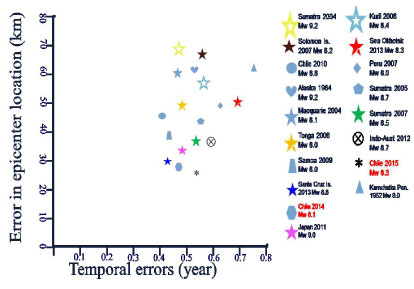
There are three interlaced mechanisms working together to make the earthquake prediction difficult for present existing rubrics. The mechanisms identified here are tested positively against 73 historical cases, all within the NCEP-NCAR reanalyses period, with high quality precipitation data. The reproduced earthquakes are close to those observed, especially for cases after 2003 (the start time of GRACE measurements) and before 2015 (the aging of the current GRACE satellites). By simulating the time scales of the evolution of strain and stress in the fault zone, using SEGMENT, with appropriate parameter settings, assisted by remote sensing information, the timing and location of major earthquakes (Mw > 5 globally) can be estimated. The uncertainties in timing are reduced to a year, and the location errors to within 120 km (the root mean squared error for historical records during 1979-2015). The primary limitation on the prediction accuracy is the resolution of the CRUST- 1.0 model, depending on which SEGMENT resolves fault geometry and composing material properties. Figure 4 is the hind-casts of historical earthquakes greater than Mw 8. It is apparent that simulation of cases within the remote sensing era has significantly smaller spatio-temporal errors. Over the same fault zone, those cases within the GRACE observational period have the smallest simulation errors. As with all prediction systems, the uncertainty grows exponentially with forecasting lead time. In the following discussion, the uncertainty level will be presented as necessary.

Although global results have been obtained for earthquake correlations with fluctuations in gravity fields resulting from groundwater discharge and extraction, the following discussion focuses on two regions: The Hikurangi subduction fault-Alpine fault-puysegur mega thrusts of New Zealand (HAP), and the Tibetan Plateau and its surrounding regions (TP, a continental collision earthquake zone). Both regions are adequately covered by GPS measurements and have adequately sizable land areas that can be sensed by GRACE for the mass fluctuations around the faults. As a result of different fault geometries, plate opposing motion speeds, and the distribution patterns of inter-plate GM, earthquakes over the selected regions are of various morphologies. Major earthquakes over the TP and HAP regions refer respectively to earthquakes of magnitudes > Mw 5.5 and Mw > 5. In the Supplementary Material (SM), applications to subduction earthquake zones are further discussed for two other earthquake-prone regions: the Andes and the Cascadian subduction zones, along with global maps of time scales of plate resonance responses to external forcing by groundwater fluctuations.

Earthquake activity in the New zealand region

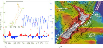
The weight of groundwater alone is unimportant as a normal pressure component in a fault. However, the lateral stress it exerts on the surrounding region is critical for fault instability. The second critical point is that, through fatigue mechanisms, groundwater extraction leaves a memory on the fault interface and forms a mechanism for temporal accumulation. Figure 5 shows the occurrence of major earthquakes over New Zealand since 1995. All major earthquakes occurred during the relatively dry periods (low groundwater levels as indicated by the low spikes in the blue curve of gravity anomalies). This high correlation is not by chance. Using SEGMENT, the transient stress field exerted by the groundwater deficit (relative to a long-term mean) is simulated for the Kaikoura Mw7.8 earthquake on November 16, 2016 (Figure 5b). Kaikoura resides in a maximum region of the R_xz stress field exerted by groundwater deficit, which reaches 5 kPa. This additional stress, even if was not the effective trigger for the major earthquake, is sufficient for triggering the following slow slip events (SSEs, personal communication with L Wallace [9]). For the events shown in Figure 5, it appears that most of the high correlations result from the groundwater deficit being an effective trigger rather than being a direct cause, even though the shear stress exerted by gravity fluctuation (groundwater extraction through net evaporation) can be orders of magnitude greater than the weight of the groundwater in the fault conditions (e.g., horizontal pushing as in the train carriage illustration in Figure 2). Also notable is that, through bridging effects and GM generation, each cycle of groundwater fluctuation leaves a 'mark' on the plate interface. This is a mechanism for the temporal accumulation of groundwater effects. From the two major mechanisms described above, many seemingly distinct earthquake events become explicable. A further examination of the 73 historical records worldwide suggests the above groundwater hypothesis likely is universally applicable.

Earthquake activity in the Tibetan plateau region

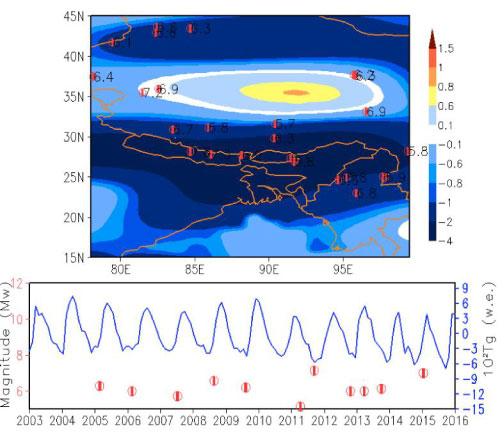
Large scale (e.g., 1000 km) groundwater fluctuations exert additional stress on a fault interface. From Figure 6, almost all major (> Mw 5.5) earthquakes during 2003-2016 over the Tibetan Plateau also occurred during low groundwater phases (Figure 6b), similar to the New Zealand cases of Sec 3.1. Although the fluctuation of groundwater is secondary to plate motion in causing stress build-up, its addition can trigger an earthquake. Analyzing the stress field clearly indicates that once two plates are coupled together, the underlying plate drags the lighter overriding plate downward and they move in tandem deeper into the Earth, pushing aside the higher density upper mantle material. This causes mass loss around the fault region. This process, although only causing mass loss at a rate of two orders of magnitude smaller than the groundwater discharge, is however, aided when the region is experiencing mass loss due to groundwater reduction (e. g., when evaporation steadily exceeds precipitation during extended droughts). The recent Nepal earthquakes of April and early May, 2015, and another, third, earthquake in Burma a year later all reside within the mass loss region. The temporal sequence of these three major earthquakes and the ruptures' spatial pattern (starting from northwest and extending to southeast) can be explained by the GM production and its transportation, as proposed here. They represent key stages of strain energy release in the lateral direction, along the transverse direction of the fault, by unlocking the granular 'sticky' spots scattered over the plate interface. The order of unlocking strictly follows the GM accumulation in the shear zone.

The three epicenter-consisting patches (comprising the three respective epicenters) all were approaching saturation by April 2015, after ~72 years of stress accumulation [34-36]. The western-most epicenter ruptured first because it was aided by groundwater reduction. Based on SEGMENT simulations, the groundwater recharge over the past 80 years has a decreasing trend over the Bay of Bengal region (74-104ºE; 15-35ºN), in agreement with the monsoonal precipitation trends identified in Ref. [37]. On average, the groundwater reduction rate was ~31 Gt/yr. This super-imposed stress field produces a saturated area (as defined in Eq. (A1)) of ~85 km2 annually. The matured (saturated) area is not spatially contiguous on the fault interface; it scattered across the inter-seismically locked interface in a complicated-connected manner. Connection of these sporadically scattered saturated patches is critical for generating earthquakes. For example, the occurrence of the first earthquake (April 25, 2015; Mw 7.8; epicenter at 28.147ºN, 84.708ºE) redistributed the granular material due underneath and established a stronger rock-rock contact, lessening the degree of saturation of the second major earthquake (May 12, 2015 of M7.3 magnitude and epicenter located 200 km to the southeast at 27.973ºN, 85.963ºE) region, so another month had passed before its occurrence. The earthquakes over Burma (Mw 6.9 on April 12, 2016 at 23.13ºN, 94.9ºE and Mw 6.8 on August 25, 2016 at 20.9ºN, 94.6ºE), further to the southeast, were not directly related to the first two earthquakes. They were a result of the lightening of the Bay of Bengal region, to be further addressed, below. Unlike some recent studies 24 predicting that the future earthquake after the Nepal earthquake of 2015 would be in the sector to the northwest, the SEGMENT simulation indicates that the sector to the south-east also is becoming unstable. In actuality, the maturation pattern jumps between the eastern and western sectors, with cluster centers at (30ºN, 84.4ºE) and (27.5ºN; 86.2ºE). Consequently, major earthquakes also occur alternatively between these two regions, in a bi-polar mode.

The LFZ is a classic example of the 'non-unique solution' configuration presented in Figure 2. The LFZ defines the eastern margin of the Tibetan Plateau. A very recent synthetic approach, using a gravity survey, seismic reflection profiles and earthquake focal mechanism data, and sediment analysis indicated that the LFZ essentially is composed of two segments of different formations. The central-northern section, which was formed ~ 40 Myr ago [38,39], is a lithospheric through-cut fault zone that is of low elastic strength but has strong dextral strike-slip motions. In contrast, the southern sector is a crustal thrust zone dominated by shallow-angle thrust motion of the TP over the moderately stiff South China Plate. This Mobius-twisted fault plane and contrasting behaviors along the LFZ, in addition to providing kinematically favourable conditions for instability, also has a profound influence on the groundwater reservoir. The Mw 7.8 Wenchuan earthquake offers further evidence of the importance of gravity field changes in fostering major earthquakes.

The mass change fields averaged over the period 2003-2008 indicate clearly that Wenchuan resides at the center of a saddle region (Figure 3 in Ref. [10]). As illustrated in the 4^th scenario train in Figure 2, the superimposed stresses form a strong compressive stress in the horizontal direction, aiding the existing geological compression. For earthquakes occurring along the same fault (but temporally consecutive), the compression caused by tectonic plate motion usually produces very similar saturation patterns. The primary reason for the randomness of epicenters is the increase in transient perturbations, such as groundwater fluctuations. The superimposed field causes a specific point to reach saturation first and then propagates away to cause a large rupture area. The rupture can grow because, to halt the motion of the unstable plates, neighboring unsaturated regions may be activated. If the propagation encounters too many unsaturated regions, the momentum is quickly lost, strongly limiting the magnitude of the earthquake. However, if the propagation starts from a region surrounded by a nearly saturated neighborhood, a positive feedback forms and is supportive of large magnitude earthquake formation. By initiating the rupture near Wenchuan, a more efficient energy release is achieved. From the SEGMENT simulations with future precipitation scenarios under the IPCC SRES A1B scenario provided by a small-volume climate model ensemble (as listed in Table 1), the next major earthquake is expected to occur in the Ganshu province (epicenter located along a 104.8ºE longitudinal arc between 33ºN and 35ºN) to the north east, ~ 120 ± 45 years later of magnitude ~ Mw7. For the far-larger TP region, the India Eurasian collisional system, while thickening the elastic lithosphere, has created numerous vertically extended crevasses. These crevasses are very effective in channeling groundwater to greater depth. Combined with the TP's orographic effects, precipitation variation transfers readily into extra lateral stress on the faults. Therefore, groundwater fluctuations become a dynamic factor affecting the epicenter location and the magnitude of major earthquakes. Because of the persistent gravity reduction in the Bay of Bengal area and Southwest China, coupled with insignificant changes over the plateau and the northern Tarim and very arid Qaidam basins, a saddle-shape super-imposed stress field has formed and has persisted over the past half century. The natural, geological, recurrence frequency (background-deduced "dry" frequency) is greatly reduced over the region, especially over the Southeast Asia peninsula. The fault zone over Myanmar likely will become unstable in approximately two years. Of great interest is that the epicenters of the upcoming earthquakes, affected by the weakening of monsoonal precipitation, are located along the 96 ± 1ºE parallel between 17-28ºN (most frequently in the 17-23ºN sector), roughly parallel to the Ayeyarwady River basin.

In addition to the pre-Himalayan and the New Zealand regions, the authors have shown that there are strong, statistically significant correlations between tectonic plate earthquake irregularities and groundwater fluctuations over many other global faults, agreeing with several recent studies (e.g., Refs. [6,7]). For example, the central Italy earthquake (August 24, 2016) and the Lorca earthquake (May 11, 2011) both occurred at low groundwater level stages. The main value of SEGMENT is its predictive ability. Previous models only involve the groundwater induced crustal unloading, or the direct mechanical effect of groundwater as in Eq. (1). Without considering the fault weakening effects from groundwater, these models explain reasonably well the observed fault slip patterns resulting from groundwater depletion. However, predicting earthquakes is beyond the capability of such models. The SEGMENT, by placing groundwater fluctuations at the nexus of all prongs of the earthquake triads, especially emphasizing the effective fault weakening from the cyclic variations of the induced crustal loading, possesses the ability to simulate the role of groundwater in future earthquakes. Using the SEGMENT modeling system, driven by precipitation scenarios from climate model projections, the future occurrence of earthquakes over the Cascadian and Andes subduction zones is investigated (in the SM). It was found that fatigue caused by groundwater fluctuations, associated with increased precipitation volatility in 21st Century California, will likely be decisive in shortening the time scale of the natural earthquake cycle of the Cascadian subduction fault (SM). However, as a consequence, their magnitudes will be reduced. For the Andes region, in addition to the regular precipitation pattern from ENSO, the granular chute system left by seamounts on the Nazca and Jun Fernandez Ridges foster major earthquakes.

Discussion

Attempts to understand earthquakes have a very long history and are globally widespread. The novel earthquake theory presented here follows from a confluence of several factors: Advances in remote sensing technology; recent, tectonically active stages motivated many researchers to re- evaluate previous assumptions [33]. Most critically, a well-documented landslide numerical model is used as a prototype of an advanced numerical modeling system to represent the mechanics of inter- plate earthquakes, and to verify the original hypotheses proposed here. This study shows, through data analysis and modeling, that variations in groundwater loading and occurrence of drought conditions together influence the occurrence and properties of earthquakes. Otherwise, the stationary seismicity of neotectonics is very stable for the majority of major faults mapped on existing neotectonic models. The temporal scale separation, i.e., the geological conditions vary at a much longer time scale than the occurrence of major earthquakes, which underscores why groundwater fluctuations constitute a viable mechanism for affecting earthquakes.

Earthquakes occur when the repose angle determined by plate-coupling stress reaches the sum of two angles representing, respectively, the fault geometry and fault strength. Accurate representation of the evolution of fault strength and repose angle therefore is critical for earthquake simulation and prediction. The earthquake triad, as defined in this study, is a generic framework that has universal applicability. Groundwater fluctuations, although relatively small, nevertheless play a pivotal role in linking the three triad components together and thereby determining earthquake irregularity. Groundwater influences fault instability directly by super-imposing a seismogenetic lateral stress field working in synergy with plate coupling stress, and also indirectly, by weakening the fault from within by enhancing fault fatigue from GM generation. The direct effect alone, the groundwater fluctuation superimposed stress field is of the same order as the residual of gravity- aided frictional stress and plate coupling stress; hence it affects the timing of major earthquakes. These findings agree with recent studies by Amos, et al. [6] and Gonzalez, et al. [7], and present the results in a coherent theoretical framework. The present study addresses the concerns of Avouac [40] and is a significant advance in understanding earthquake dynamics and thermodynamics for reliable earthquake prediction.

By exploring existing records of earthquakes using SEGMENT, it is found that for collisional systems, direct effects from groundwater control the irregularity of major earthquakes. Essentially, the orographically highly variable precipitation is effectively channeled into deeper depth by the prevalence of through-cut faults. Droughts elsewhere also are seismogenetic but likely their effects are indirect. For example, the Elnino-southern oscillation (ENSO), as the dominant climate driver of regional precipitation, has a strong influence on the gravity field over the Andes region of South America. The occurrence of major earthquakes, although bearing the same 4-7 year occurrence frequency of ENSO, has a significant hiatus when compared with the fluctuation in the gravity field. Similarly, the stability of the Cascadia fault is found to be remotely affected by Californian droughts. The input of strain energy from the periodic recharge and discharge of groundwater in a large regional area increases the prospect of un-locking of seismically coupled plates. Thus, climate fluctuations can and do determine the groundwater loading pattern through extended droughts and extreme precipitation storms, which in turn affect the earthquake cycles. The actual impacts of a warming climate are fault specific, but for the San-Andreas Fault, located in a Mediterranean climate zone, an enhanced hydrological cycle will further reduce the magnitude of earthquakes but enhance the occurrence frequency.

Existing geological data limited SEGMENT only represent major faults on orogens. Large number of minor faults [41,42] are not included in the input data, and their seismic activity in those locations are beyond the capability of our modeling system. New higher resolution geodetic information on plate interface and boundaries, sea floor spreading, fault systems, and geodesy all are necessary for further improvements of the predicting score, by improved description of continuum deformation and subsequent rupture/yielding.

Supplementary Materials

Due to size limitation, important details are provided in the Supplementary Material (SM). The author also will provide assistance if readers wish to re-produce the results.

Conflicts of Interest

The authors declare no competing financial interests.

References

1. Scholz C (1998) Earthquakes and friction laws. Nature 391: 37-42.
2. Wang K, Hu Y (2006) Accretionary prisms in subduction earthquake cycles: The theory of dynamic Coulomb wedge. J Geophysical Res 111: 410.
3. Wang K, He J (1999) Mechanics of low-stress forearcs: Nankai and Cascadia. J Geophysical Res 104: 15191-15205.
4. Bercovici D, Ricard Y (2014) Plate tectonics, damage and inheritance. Nature 508: 513-516.
5. Liu Z, Bird P (2008) Kinematic modelling of neotectonics in the Persia-Tibet-Burma orogen. Geophys J Int 172: 779-797.
6. Amos CB, Audet P, Hammond WC, et al. (2014) Uplift and seismicity driven by groundwater depletion in central California. Nature 509: 483-486.
7. Gonzalez P, Tiampo K, Palano M, et al. (2012) The 2011 Lorca earthquake slip distribution controlled by groundwater crustal unloading. Nature Geoscience 5: 821-825.
8. Koketsu K, YusukeYokota, Naoki Nishimura, et al. (2011) A unified source model for the 2011 Tohoku earthquake. Earth Planet Sci Lett 310: 480-487.
9. Wallace L, Susan Ellis, Paul Mann (2009) Collisional model for rapid fore-arc block rotations, arc curvature, and episodic back- arc rifting in subduction settings. Geochem Geophys Geosyst 10: Q10006.
10. Ren D, Lance M Leslie, Xinyi Shen, et al. (2015) The gravity environment of Zhouqu debris flow of August 2010 and its implication for future recurrence. International J Geo 6: 317-325.
11. Gao X, Wang K (2014) Strength of stick-slip and creeping subduction megathrusts from heat flow observations. Science 345: 1038-1041.
12. Wang K, Hu Y, He J (2012) Deformation cycles of subduction earthquakes in a viscoelastic earth. Nature 484: 327-332.
13. Jop P, Forterre Y, Pouliquen O (2006) A constitutive law for dense granular flows. Nature 441: 727-730.
14. Ren D, Leslie L, Karoly D (2008) Mudslide risk analysis using a new constitutive relationship for granular flow. Earth Interactions 12: 1-16.
15. Bejar-Pizarro M, Anna Socquet, Rolando Armijo, et al. (2013) Andean structural control on interseismic coupling in the North Chile subduction zone. Nature Geoscience 6: 462-467.
16. Ren D, Leslie L (2014) Effects of waves on tabular ice-shelf calving. Earth Interactions 18: 1-28.
17. Famiglietti J, Rodell M (2013) Water in the balance. Science 340: 1300-1301.
18. Ren D (2014) The devastating Zhouqu Storm-triggered debris flow of August 2010: Likely causes and possible trends in a future warming climate. J Geophys Res 119: 3643-3662.
19. Voss KA, Famiglietti JS, Lo M, et al. (2013) Groundwater depletion in the Middle East from GRACE with implications fo transboundary water management in the Tigris-Euphrates-Western Iran region. Water Resour Res 49: 904-914.
20. Ren D (2014) Storm-triggered Landslides in warmer climates. Springer, NY.
21. Ren D, Leslie L, Lynch M (2012) Verification of model simulated mass balance, flow fields and tabular calving events of the Antarctic ice sheet against remotely sensed observations. J Clim Dyn 40: 11-12.
22. Laske G, Masters G, Ma Z, et al. (2013) Update on CRUST1.0 - A 1-degree global model of earth's crust. Geophys Res Abstracts 15.
23. Martin Kronbichler, Timo Heister, Wolfgang Bangerth (2012) High accuracy mantle convection simulation through modern numerical methods. Geophysics Journal International 191: 12-29.
24. Field E, Biasi G, Bird P, et al. (2013) Uniform California earthquake rupture forecast, version 3 (UCERF3)-The time-independent model. US Geol Surv 104: 1122-1180.
25. Van der Veen C, Whillans I (1989) Force budget: I. Theory and numerical methods. J Glacio 35: 53-60.
26. (2006) Andes Geological Survey.
27. Lay T (2015) The surge of great earthquakes from 2004 to 2014. Earth and Planetary Science Letters 409: 133-146.
28. Kreemer C, Holt W, Haines A (2003) An integrated global model of present-day plate motions an plate boundary deformation. Geophys J Int 154: 8-34.
29. Liu Z, Bird P (2002) Finite element modeling of neotectonics in New Zealand. J Geophys Res 107: 2328.
30. Timoshenko S, Gere J (1963) Theory of elastic stability. McGraw-Hill, New York.
31. Gilman J (2004) Direct measurements of the surface energy of crystals. J Appl Phys 31: 2208.
32. Dietrich W, Perron J (2006) The search for a topographic signature of life. Nature 439: 411-418.
33. Wang K (2015) Subduction faults as we see them in the 21st Century. AGU Birch Lecture.
34. Ummenhofer C, England M (2007) Interannual extremes in New Zealand precipitation linked to modes of 747 Southern Hemisphere climate variability. J Climate 20: 5418-5440.
35. Men K, Zhao K (2016) The 2015 Nepal M8.1 earthquake and the prediction for M ≥ 8 earthquakes in west China. Natural Hazards 82: 1767-1777.
36. Bollinger L, Sapkota SN, Tapponnier P, et al. (2014) Estimating the return times of great Himalayan earthquakes in eastern Nepal: Evidence from the Patu and Bardibas strands of the main frontal thrust. J Geophysical Res 119: 7123-7163.
37. Wang B, Ding Q (2006) Changes in global monsoon precipitation over the past 56 years. Geophysical Res Lett 33: L06711.
38. Jiang XD, Li ZX (2014) Seismic reflection data support episodic and simultaneous growth of the Tibetan Plateau since 25 Myr. Nature Communications 5: 5453.
39. Richardson N, Densmore AL, Seward D, et al. (2008) Extraordinary denudation in the Sichuan Basin: Insights from low-temperature thermochronology adjacent to the eastern margin of the Tibetan Plateau. J Geophysical Res 113: B04409.
40. Avouac J (2012) Earthquakes: Human-induced shaking. Nature Geoscience 5: 763-764.
41. Taylor M, Yin A, Ryerson F, et al. (2003) Conjugate strike-slip faulting along the Bangong-Nujiang suture zone accommodates coeval east-west extension and north-south shortening in the interior of the Tibetan Plateau. Tectonics 22: 1044.
42. Pollastro R, Karshbaum A, Viger R (1998) Map showing geology, oil and gas fields, and geologic provinces of Iran. USGS Open File Report 97: 470.
43. Rowe C, Kirkpatrick J, Brodsky E (2012) Fault rock injections record paleo-earthquakes. Earth and Planetary Science Letters. Earth and Planetary Science Letters 335-336: 154-166.
44. Ujjie K, Asuka Yamaguchu, Gaku Kimura, et al. (2007) Fluidization of granular material in a subduction thrust at seismogenic depth. Earth Planet Sci Lett 259: 307-318.
45. Cowan D, Cladouhos T, Morgan J (2003) Structural geology and kinematic history of rocks formed along low-angle faults, Death Valley, California. Geol Soc Am Bull 115: 1230-1248.
46. Chlieh M, Perfettini H, Tavera H, et al. (2011) Interseismic coupling and seismic potential along the Central Andes subduction zone. J Geophys Res 116: 12.
47. Sun T, Wang K, Linuma T, et al. (2014) Prevalence of viscoelastic relaxation after the 2011 Tohokuoki earthquake. Nature 514: 84-87.
48. Loveless J, Meade B (2010) Geodetic imaging of plate motions, slip rates, and partitioning of deformation in Japan. J Geophys Res 115: B09301.
49. Cavalie O, Jonsson S (2014) Block-like plate movements in eastern Anatolia observed by InSAR. Geophys Res Lett 41: 1-6.
50. Weston J, Ferreira A, Funning G (2012) Systematic comparisons of earthquake source models determined using InSAR and seismic data. Tectonophysics 532-535: 61-81.
51. Wang K, Bilek S (2011) Do subducting seamounts generate or stop large earthquakes. Geology 39: 819-822.
52. Pritchard M, Simons M (2006) An aseismic slip pulse in northern Chile and along-strike variations in seismogenic behavior. J Geophys Res 111: 8.
53. Sawai Y, Satake K, Kamataki T, et al. (2004) Transient uplift after a 17th-century earthquake along the Kuril subduction zone. Science 306: 1918-1920.
54. Baby P, Rochat P, Mascle G, et al. (1997) Neogene shortening contribution to crustal thickening in the back arc of the Central Andes. Geology 25: 883-886.
55. Christensen N, Mooney W (1995) Seismic velocity structure and composition of the continental crust: A global view. J Geophys Res 100: 9761-9788.
56. Yanez G, Ranero C, Huene R, et al. (2001) Magnetic anomaly interpretation across the southern centra Andes (32°-34°S): The role of the Juan Fernandez Ridge in the late Tertiary evolution of the margin. J Geophysical Res 106: 6325-6345.
57. Yuan X, Sobolev S, Kind R (2002) Moho topography in the central Andes and its geodynamic implications. Earth and Planetary Science Letters 199: 389-402.
58. Ren D, Fu R, Leslie L, et al. (2011) Predicting storm-triggered landslides. Bull Amer Met Soc 92: 129-139.