Journal of Aerospace Engineering and Mechanics

Mathematical Modelling and Comparative Numerical Simulations of Swing-Fuselage Junction Vortex Structures

Abstract

Turbulence and flow disturbances occurring at the aircraft wing-fuselage junction cause a deterioration of its aerodynamic performance and an increase in the aircraft's drag force. However, the aircraft junction regions are currently designed empirically due to the lack of knowledge of detailed junction flow dynamics, which consequently leads to less efficient flow management and poorer aerodynamic characteristics. The main objective of the present mathematical- modelling study is research on an aerodynamically enhanced design approach, concerning the improvement of the characteristics of the junction flow and its vortices. Numerical simulations are performed under the prism of vortices' structure formation and patterns, particularly of the horseshoe and corner separation vortices, which dominate such flows. More specifically, this research study proposes a new junction flow parameter, which has been employed in combination with the existing ones, in order to result in a more streamlined and efficient junction design, and investigates the junction flow response, when the reference junction design of a wing-fuselage system is modified by the addition of "fillet", "strake" and "blending" geometry types on the wing. Flow simulations are performed in steady-state mode, at transonic flight regime and at 2° angle of attack, using two turbulence models: The Reynolds Averaged Navier-Stokes (RANS) SST k-ω turbulence model, enhanced with rotation/curvature corrections (SST-CC) and with eddy viscosity and turbulence production limiters, and the second-order closure Reynolds Stress model. The geometrical modifications that were implemented proved to be efficient and their application in the design process of modern aircraft foreshadows the possibility of achieving enhanced-performance flights. More specifically, all the three modifications of the reference geometry increased the aircraft's aerodynamic efficiency, by improving the flow pattern around the wing-fuselage regions at the studied flight state. The most promising configuration proved to be the one which combined the "fillet" and "strake" geometries, resulting in the highest aerodynamic efficiency, by greatly weakening the horseshoe vortex and eliminating the corner separation.

Keywords

CFD, Junction flows, SST-CC, Vortex structures, Fillet, Strake

Nomenclature

The following symbols are used in this paper:

Br- Brinkman number

B.F. - bluntness factor

B.O.I- body of influence

c- Chord length

$c_{r1}$ - Additional empirical constant in the SST-CC model = 1.0

$c_{r2}$ - Additional empirical constant in the SST-CC model = 2.0

$c_{r3}$ - Additional empirical constant in the SST-CC model = 1.0

Cd- Drag coefficient

Cl- Lift coefficient

Cl/Cd- Aerodynamic efficiency

Cp- Pressure coefficient

$C_{scale}$ - Coefficient related to the strength of the curvature correction = 1.0

$\frac{D{S}_{ij}}{Dt}$ - Components of the Lagrangian derivative of the strain rate tensor

$D_{\omega }$ - Cross-diffusion term

${\tilde{f}}_r$ - SST k- ω model empirical curvature correction function

$f_r$ - SST k- ω model production term multiplier - curvature correction function

$f_{rotation}$ - Spalart-Allmaras model empirical curvature correction function

$G_k$ - Production of k with the production limiter

$G_{\omega }$ - Production of ω

I.S.A- International Standard Atmosphere

k- Turbulence kinetic energy

LES- Large eddy simulation

M.D.F.- momentum deficit factor

$\tilde{r}$ - Argument of

$r^{*}$ - Argument of

${\mathrm{Re}}_T$ - Reynolds number based on the wing's thickness

${\mathrm{Re}}_{{}_{\theta }}$ - Reynolds number based on the boundary layer momentum thickness

$R_o$ - Leading edge radius

RANS- Reynolds-averaged Navier-Stokes

RSM- Reynolds Stress Model

S - Strain rate magnitude

$S_{ij}$ - Components of strain rate tensor

$S_k$ - Source term

$S_{\omega }$ - Source term

$S_T$ - Distance from the leading edge along the airfoil surface to the maximum thickness

SST- Shear stress transport

SST-CC- Shear stress transport k-ω model with rotation/curvature corrections

T- Maximum thickness of the wing

u- Local velocity

u+- dimensionless velocity

u*- friction velocity

u□ -velocity component

U- free stream velocity

v- kinematic viscosity

X□- spatial component

$X_T$ - Chord wise location of T

y⁺- Dimensionless distance

$Y_k$ - Dissipation of k

$Y_k$ - Dissipation of ω

z- Longitudinal axis

□ -axis direction

3D- three dimensional

${\beta }_{\infty }^{*}$ - Constant in the standard k-ω model = 0.09

${\beta }_i$ - Coefficient in the SST k-ω model

${\tau }_k$ - Effective diffusivity of k

${\tau }_{\omega }$ - Effective diffusivity of ω

$\delta$ - Boundary layer thickness

$\Delta T$ - Difference of temperature between two measuring points

${\epsilon }_{imn}$ - Tensor of Levi-Civita

θ - Momentum thickness

$K_{thermal}$ -Thermal conductivity

μ- Molecular viscosity

ρ- Fluid's local density

ρ₀ - Free stream density

ω - Specific dissipation rate

${\omega }_w$ - Specific dissipation rate at wall

$\Omega$ - Vorticity magnitude

$\Omega$ - Vorticity magnitude

${\Omega }_{ij}$ - Components of vorticity tensor

${\Omega }_m^{rot}$ - Components of the system rotation vector

Introduction

Aerodynamic performance in the design of the commercial aircraft has always been a crucial goal for the aircraft designers. The wing-body junction is an area of additional drag, where designers implement modifications in order to minimize the drag force and maximize the aircraft's aerodynamic efficiency. Wing-fuselage, tail-fuselage and pylon-nacelle are some of the aircraft's junctions. Junction flows happen when an incoming boundary layer encounters an obstacle. These flows are known for being rich in flow physics, since they are highly strained, anisotropic and strongly affected by unsteady turbulence.

For the aircraft's wing-fuselage junction flow, where the Reynolds number is reasonably high, the adverse pressure gradient, which is induced by the presence of the wing, leads to the upwind boundary layer separation, forming one or multiple horseshoe vortices. The horseshoe vortex can be classified as first kind secondary flow according to Prandtl, because it is linked to the skewing of the mean flow [1]. Many researchers characterize the horseshoe vortex as the dominant vortex structure at the junction flow. However, mixing of fuselage and wing's boundary layers forms a corner boundary layer, which has to overcome the adverse pressure gradient imposed by the wing as well as the wall friction of the wing and the fuselage. This combined with the horseshoe vortex effect, may result in the occurrence of a premature corner separation. The horseshoe vortex is not the only vortex that appears in junction flows, but there also exist some relatively weaker secondary vortices, which commonly energize the low-momentum region in the corner flow, decreasing the tendency towards separation [2].

The surface of junctions can be smoothed by modifying its shape, in order to achieve a more desirable flow characterized by horseshoe vortex elimination and corner separation prevention. Notwithstanding the foregoing, these modifications are made empirically by aircraft designers, due to the lack of knowledge of junction flow dynamics and especially of corner separation occurrence. In this paper we present the study of "fillet", "strake" and "blending" types of such geometrical design modifications.

For junction flows, there are until now studies for a limited number of parameters that characterize the behavior of the junction flow and, therefore, there is need to identify more parameters that affect the formation of the junction flow region. As far as the reported in literature parameters are concerned, Fleming, et al. [3] introduced an indicator of the strength of the horseshoe vortex, which highlights the critical role of the wing's leading edge shape [4,5], called the "Bluntness Factor" and another parameter of junction flows, called "Momentum Deficit Factor" [6]. The B.F. indicates that round leading-edge shapes create stronger horseshoe vortices, as opposed to the sharp ones. This M.D.F. is linked to the distortion of the axial velocity, as characteristic of incoming boundary layers. For high values of this parameter, there is higher velocity distortion in the junction flow and the horseshoe vortex legs come closer to the wing's surface. Khan, et al. [7-9], also takes into consideration the influence of wing's sweep. According to the results of those studies, sweep tends to attenuate the strength of the horseshoe vortex. Specifically, backswept wings tend to lift up the horseshoe vortex and bring the legs closer to the wing's surface. On the contrary, forward swept wings tend to push the horseshoe's core and the legs away from the wing's surface.

It has become apparent that horseshoe vortex and corner separation are likely to co-exist within a junction. It should be mentioned that the most recent and advanced experimental dataset dedicated to the corner separation analysis was carried out by NASA Juncture Flow validation case [10-16]. There are also some other test cases examined that focus mainly only on the horseshoe vortex characteristics, which are commonly referred to the Rood's wing case (named after its designer, E.P. Rood) or to flat plate-wing configurations. Therefore, in the present study, it was considered necessary to examine specifically the junction flow. The test case considered for the mathematical modelling and computer simulation was the junction flow around a 1/10 scaled 150-passenger airliner, focusing on the formation of vortices and investigating possible other parameters that may affect the junction flows.

Despite the continuously developing knowledge on understanding the junction flows behavior, the literature of the public domain focuses mainly on lower Reynolds numbers and lower Mach numbers than those of the cruise flight of a typical airliner. Furthermore, limited configurations and a very restrictive range of M.D.F. and B.F. are researched (for example the standard DLR-F6 and others - see Table 6 below). The present authors, therefore, orientated their investigation towards other unexplored flow conditions and configurations and undertook numerical investigation research on those topics. Additional elements that have been considered are the curvature of the fuselage configuration at the junction region, which is a critical parameter for the development and the evolution of the formed vortices at the leading edge of the wing at the junction region, in contrast with the configurations of the public domain that use flat or flattened fuselage surfaces at the junction plane. Any other wing and fuselage combination that meets the study criteria could have been chosen of course, but the main interest of this work is directed towards improving the aerodynamic and flow characteristics of the junction region. This is done via researching the possibilities of applying shaping-modification techniques on that region and investigating the way that the formed vortices interact with the main flow in each case. The reported work configurations give the opportunity to investigate B.F. and M.D.F. combinations that are not reported in the literature to-date.

Mathematical Modelling

Governing equations and turbulence modelling

The governing equations for the wing- fuselage junction steady flow are the three-dimensional, steady- state, compressible Reynolds Favre-averaged Navier-Stokes (RANS) equations, expressed in curvilinear non-orthogonal coordinates. These equations are very well known and are not repeated here [17-20].

Although the actual problem is the analysis of the vortices, where an unsteady 3D model could have been used, the computational demands for such a case are very restrictive. The steady-state results give, in general, a good approximation, in a comparative manner, of the overall consequences of the proposed configurations and useful results may be obtained, within practical resources, at least for engineering design purposes. After all, turbulence is always an unsteady phenomenon, yet very practical results have been obtained to-date for important engineering applications, run under steady-state conditions.

Several articles demonstrate the need for non-linear -closure turbulence models [21-29] for junction flow investigations, where corner separation is present. For this reason two turbulence models were used in the present work, the SST (Shear Stress Transport) k-ω model [20,30-34], appropriately modified for the purpose of this work, and the second order Reynolds-Stress Model (RSM) [33-35]. The latter was applied since Brito Lopes, et al. [35] justify its use in problems of highly swirling flows and complex geometries.

As it will be shown, in the results section below, the difference in predictions by the two models is minor and does not warranty the seven-fold increase in computational time required by the second order model. Therefore, the results presented and discussed are the ones with the modified SST k-ω model.

The chosen model is a 2-equation model, which is considered reliable and is commonly used in sophisticated aerospace applications, for flows with adverse pressure gradients, separation and shock waves at transonic flow regimes. Apart from its reliability in aerospace applications, Snigha, et al. [36] highlight its congruent results when predicting the flow separation at the wing-fuselage junction. However, in the present study, the SST k-ω model was not used in its original form. Specifically, aiming towards more accurate computational results in the junction region, this turbulence model was enhanced taking into account rotation/curvature corrections (SST-CC) [34], as well as compressibility corrections and the viscous heating effect, in order to improve accuracy for the transonic flight regime. Eddy viscosity and turbulence production limiters, as well as the Kato-Launder modifications are also properly applied to adapt the turbulence model to the present physical test case, in order to prevent the spurious build-up of turbulence in stagnation regions and the turbulence viscosity over prediction. The above modifications lead to improved predictions, comparable with second-order closures, as observed in the present study as well as in Kato and Launder [37]. The Kato-Launder modification is considered crucial to be employed in the junction flow study, since it has beneficial effects on flows with rotation and swirl, as compared to the original model, predicting more accurately the junction flow features.

Despite the fact that the SST k-ω model may still fail to account for more subtle interactions between turbulence stresses and mean flow, when compared with the Large Eddy Simulation (LES) or even the RSM models, even if not observed for the latter in this work for the design variables considered, it appears that for the geometries studied, the fact that the angle of attack is small (2°) and the RANS were applied at steady state, the predictions of the modified SST k-ω model remain valid and useful from a designer's point of view. Specifically, the parametric study with the two models showed that the results were similar and the types of the vortex structures were the same in all cases. Even for the corner separation cases, both models predicted the corner separation presence or absence at the same configurations, verifying that they occur due to the junction geometry and not due to the turbulence- modeling's non -linearity's. This finding justifies the design objectives of this study, in order to obtain useful results concerning the junction flow response to the junction region design modifications. This conclusion can be also supported by the current literature that indicates the SST k-ω tendency to over predict corner separations at junction flows, and at the same time that the RSM can dramatically under predict the separation size [28]. The above findings make the authors confident to conclude about the corner separation occurrence, but of course not about its exact size. Furthermore, the results are aligned with Smirnov and Menter [34], who underline the accuracy improvements because of the rotation/curvature corrections on the original SST k-ω model and the model's competitiveness with the RSM model in complex three-dimensional flows, since it is acceptably accurate but at the same time significantly more computationally efficient and robust than the latter. Finally, it should also be mentioned that the rotation/curvature correction factors introduced here are also proposed by K. Zore, et al. [38] in the junction flow simulations, since the SST k-ω option of rotation/curvature correction can effectively decrease the eddy viscosity in areas of overly complex flow structures, such as junction flows. The positive effect of the rotation/curvature correction in junction flows is also mentioned in CL Rumsey, et al. [10-39], for the quadratic constitutive relation form of Spalart-Allmaras turbulence model.

The final form of the transport equations for the SST k-ω model, including the rotation/curvature corrections (SST-CC), the compressibility corrections, the viscous heating effect, the production limiter and the Kato-Launder modification is the following:

$$\frac{\partial }{\partial t}\left(\rho k\right)+\frac{\partial }{\partial Xj}\left(\rho kuj\right)=\frac{\partial }{\partial Xj}\left(\Gamma k\frac{\partial k}{\partial {\rm X}j}\right)+Gkfr-Yk+Sk\text{ (1)}$$

$$\frac{\partial }{\partial t}\left(\rho \omega \right)+\frac{\partial }{\partial Xj}\left(\rho \omega uj\right)=\frac{\partial }{\partial Xj}\left(\Gamma \omega \frac{\partial \omega }{\partial {\rm X}j}\right)+G\omega fr-Y\omega +S\omega \text{ (2)}$$

Concerning the rotation/curvature correction that has been introduced in this work [34]:

$$fr=\max \left\{0.1+\mathrm{Csc}ale(\tilde{f}r-1)\right\}\text{ (3)}$$

Where,

$$\tilde{f}r=\max \left\{\min (frotation,1.25),0.0\right\}\text{ (4)}$$

$$frotation=\left(1+cr1\right)\frac{2r*}{1+r*}\left[1-cr3{\tan }^{-1}\left(cr2\tilde{r}\right)\right]-cr1\text{ (5)}$$

$$r*=\frac{S}{\Omega }\text{ (6)}$$

$$\tilde{r}=2\Omega ikSik\left[\frac{DSij}{Dt}+\left(\epsilon imnSjn+\epsilon jmn\mathrm{Sin}\right){\Omega }_m^{rot}\right]\frac{1}{\Omega D^3}\text{ (7)}$$

$$Sij=\frac{1}{2}\left(\frac{\partial ui}{\partial xj}+\frac{\partial uj}{\partial xi}\right)\text{ (8)}$$

$$\Omega ij=\frac{1}{2}\left(\left(\frac{\partial ui}{\partial xj}-\frac{\partial uj}{\partial xi}\right)+2\epsilon mji{\Omega }_m^{rot}\right)\text{ (9)}$$

$$S^2=2SijSij\text{ (10)}$$

$${\Omega }^2=2\Omega ij\Omega ij\text{ (11)}$$

$$D^2=\max \left(S^2,0.09{\omega }^2\right)\text{ (12)}$$

Finally, the viscous heating has been taken into account in the energy equation. Specifically, the energy equation includes the viscous dissipation terms because they are not negligible, since the Brinkman number (13) exceeds unity [40].

$$Br=\frac{\mu u^2}{\kappa therma{l}^{\Delta {\rm T}}}\text{ (13)}$$

In the aforementioned equations the Einstein summation convention is used. More details about the SST-CC model may found in P.E. Smirnov and F.R. Menter [34] and its difference with the original SST k-ω model can be found in F.R. Menter, et al. [32] and W. Malalasekera and H.K. Versteeg [20]. As aforementioned, the transport equations are enhanced with compressibility and viscous heating, eddy viscosity and the turbulence production limiters, as well as the Kato-Launder modifications [30,37,40]. The k and ω transport equations are solved simultaneously with the three momentum Navier-Stokes equations together with the continuity and energy equations, a total of 7 differential equations. This set of equations is solved using the finite-volume technique, details of which may be found in literature [20,41-43]. More specifically, the equations are transformed to curvilinear body-fitted-coordinate form and are solved as in Galea and Markatos [44] and in Spyridakos, et al. [45].

Wall boundary conditions

In the modified SST k-ω model used in the current study, the boundary conditions for the k-equation are treated by an enhanced wall treatment [40]. In that way, all the boundary conditions for wall-function meshes will correspond to the wall function approach, while for the fine meshes, the appropriate low-Reynolds number boundary condition will be applied.

The value of ω at the wall is specified as:

$$\omega w=\frac{\rho {\left(u_{*}\right)}^2}{\mu }{\omega }^{+}\text{ (14)}$$

For the laminar sublayer:

$${\omega }^{+}=\frac{6}{\beta i{\left(y^{+}\right)}^2}\text{ (15)}$$

and for the logarithmic region:

$${\omega }^{+}=\frac{1}{\sqrt{{\beta }_{\infty }^{*}}}\frac{d{u}_{turb}^{+}}{d{y}^{+}}\text{ (16)}$$

So, a wall treatment for the ω-equation is defined, which switches automatically from the viscous sublayer formulation to the wall function, depending on the grid.

Numerical simulation

The computations were performed with the ANSYS Fluent software [40], appropriately modified and adapted for the cases studied. This code has been extensively validated against experimental results for many similar, but admittedly simpler cases, and its predictions were found satisfactory.

The differential equations were solved using a cell-centered finite volume method on hybrid grids [20] and the system of the algebraic equations is solved in a coupled iterative manner. Therefore, the velocity and pressure fields are updated together. To obtain fast and smooth solution convergence, relaxation of the false-transient type [20] is used for all the variables. Using the above parameter, the convergence was smooth and monotonic, while the runs were stopped when accuracy of 10-3 for the normalized variables was achieved. A second-order upwind spatial discretization scheme was employed for all variables and the gradient was computed with the cell-based least squares method.

A typical run for a full typical simulation using the modified SST k-ω model was demanding about 8 hours CPU time for a grid of 22 million cells; and the RSM about 56 hours CPU time, in a computer system with an i9-9900k CPU and 64GB RAM, when the whole CPU was utilized in parallel processing with 8 processors.

The Test Cases Considered

Reference geometry and applied wing's modifications

The present study involves the designs with 4 different types of washout-twisted wing-fuselage junctions. These data are considered for the present research work because they are the standards for a 150-passenger commercial airliner aircraft. The modifications are based on the reference geometry, and they are associated only with the wing and the wing-fuselage junction shape. Each wing-fuselage system modification is designed in a way that includes the modifications of the previous configuration, starting from the reference geometry system. In that way, the kind of each modification is isolated and qualitative and quantitative results about each modification's effects are exported.

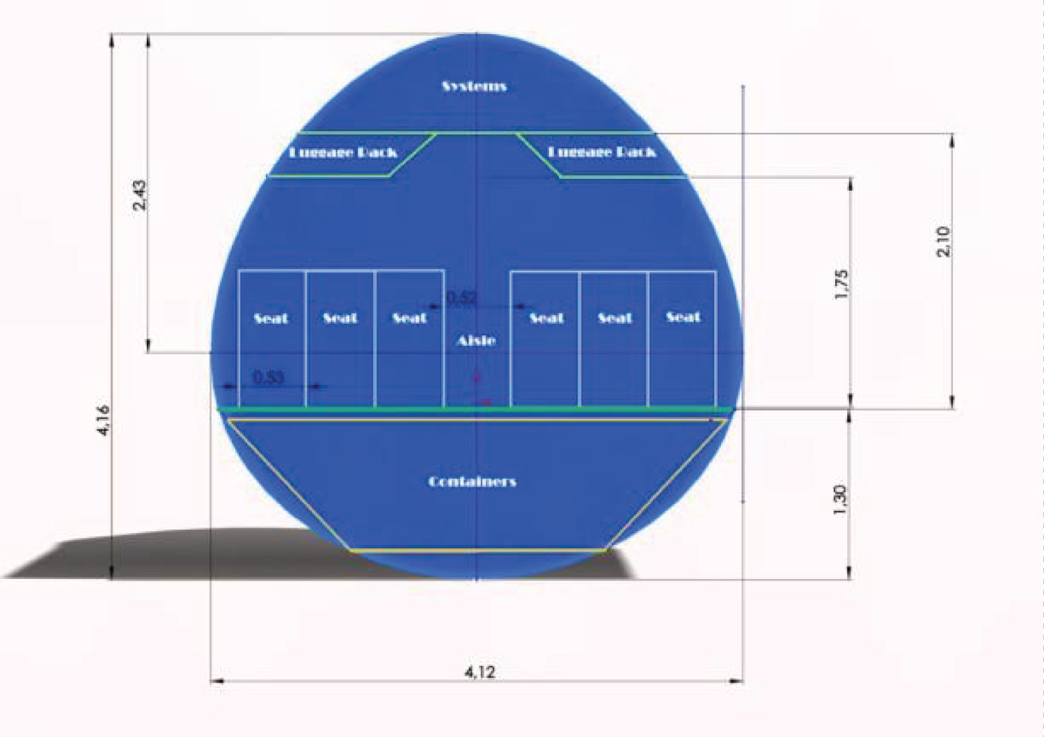
The fuselage is common for all the configurations and it is designed according to the 150-passenger capacity requirements under the comfort conditions of the modern industry [46], but also according to aerodynamic concerns under the restrictions of the former requirements [47-49] (Figure 1).

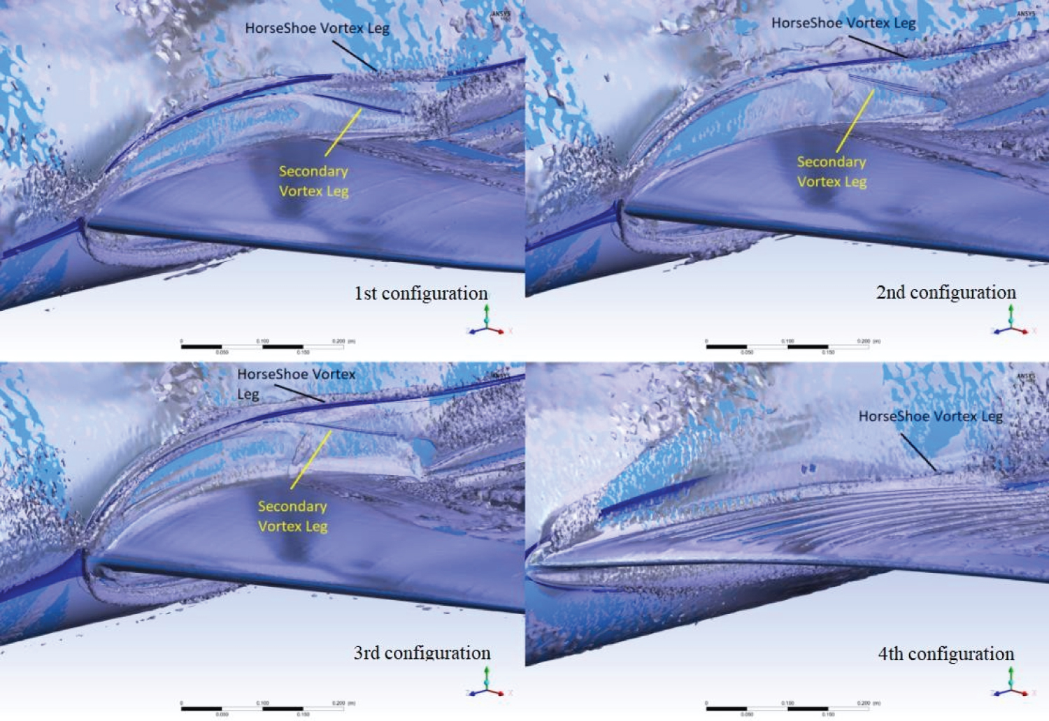
The 1^st configuration, which is used as the reference geometry, represents a typical 150-passenger mid-wing airliner aircraft. For the 2^nd configuration, the wing is connected with the fuselage in the same way as in the 1^st configuration, but the wing of the 2^nd configuration is blended and, as a result, the leading and trailing edge sweep angle is variable. It should be mentioned that the 2^nd configuration has a slightly negative trailing edge sweep angle at the root; in order to investigate if that may affect the prevention of the probable corner separation. The 3^rd configuration is exactly the same as the 2^nd configuration, with the only difference being that the 3^rd configuration's wing is connected with the fuselage via a constant 0.3m- radius fillet. At the 4^th configuration, the strake geometry at the wing has been included, combined with constant 0.2m- radius fillet connection with the fuselage. From the last two configurations we can investigate, respectively, the effect of inserting fillet and strake geometries at junction flows (Figure 2).

Computational domain and boundary conditions

The simulated geometry has a symmetry plane, which allows only half the aircraft to be studied, in order to reduce significantly the computational cost. Concerning the medium, the air is treated as ideal gas, whose laminar viscosity changes according to the Sutherland law and its properties are taken from the I.S.A (International Standard Atmosphere). The Mach number of the test case is 0.82 and the flow is studied at 2° angle of attack.

Boundary conditions

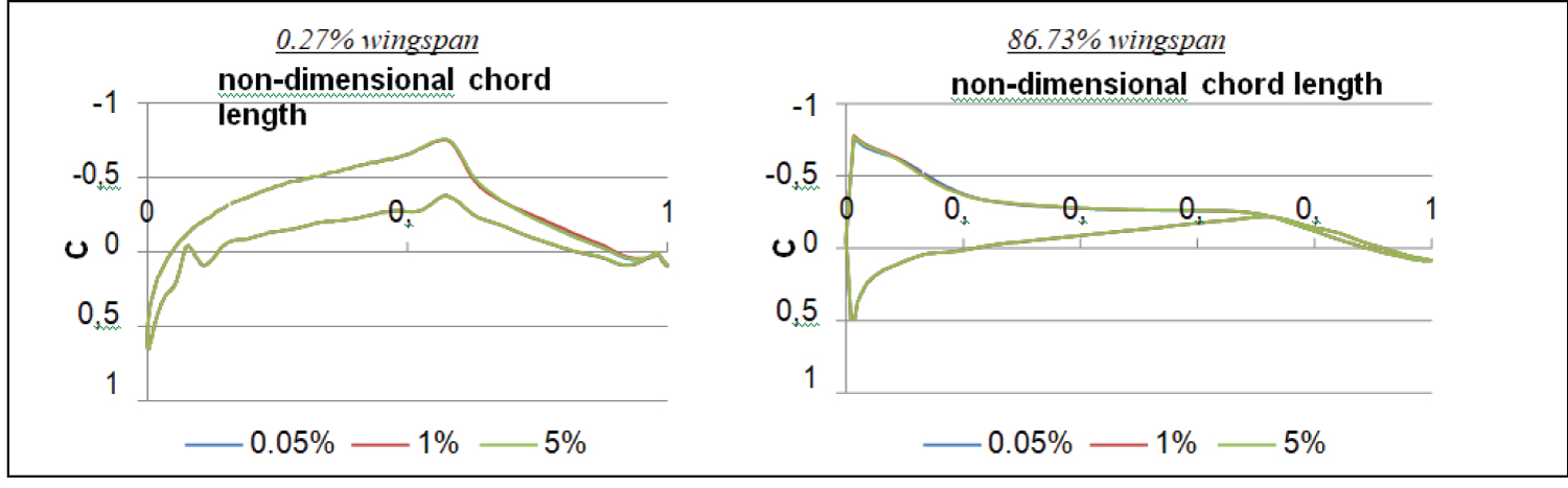
• Inlet: The inlet velocity of the flow is specified at 245 m/s at 2° angle of attack. The temperature is set to 223 K according to I.S.A. at the test case's flight altitude. The turbulence intensity is 5% and the turbulence/laminar viscosity ratio at inlet is set to 100. A turbulence intensity parametric study was performed for three turbulence intensity values, 0.05%, 1% and 5% and the results did not change. The same was true when using turbulence/laminar viscosity ratios of 300 and 500. Two typical examples are given for the junction section and the outer wing in Figure 3.

• Outlet: A specified exhaust pressure at the surrounding atmosphere is specified. At this pressure far-field boundary, a regime of 0.82 Mach at 2◦ angle of attack has been specified. As mentioned earlier, the temperature is set also at 223 K.

• Wall: The aircraft is defined as a stationary wall, demanding the no-slip shear condition. The near wall boundary treatment is defined by ANSYS Fluent for the SST k-ω model, which automatically switches from a low-Reynolds number formulation to a wall function treatment [17], based on the grid density [45].

• Free-stream boundary: The gauge pressure at the free-stream boundary of the flow is set to zero, the turbulence intensity is 5% and the turbulence/laminar viscosity ratio is equal to 100.

• Symmetry plane: The zero-gradient condition for all variables is applied at the symmetry plane.

Computational grid

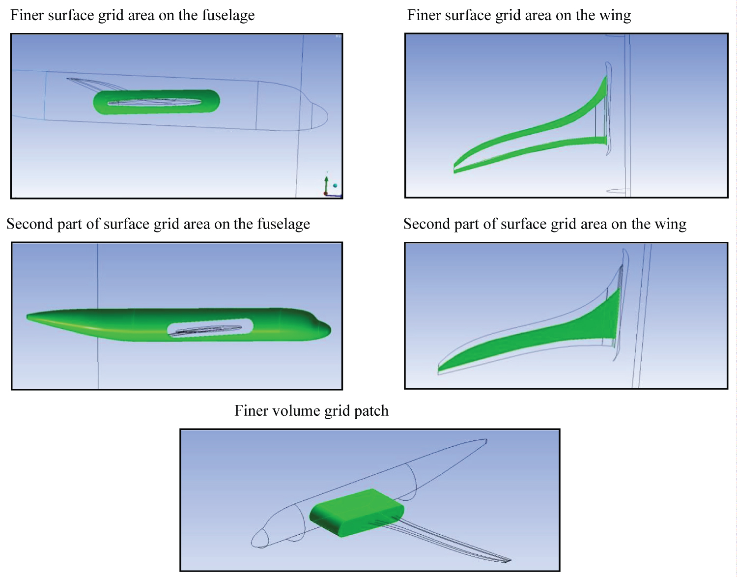
Meshing is carried out using ANSYS Meshing software. The grids of the present simulations are all hybrid, comprising prismatic layers and unstructured tetrahedral elements. Specifically, near the wall boundary layers use is made of prismatic layers to capture the boundary layer flow. The rest of the domain is discretized into tetrahedral elements, whose size gradually increases as the distance from the wall boundary increases. Additionally, some regions of higher grid's density were introduced in order to allow detailed computational information of the wing-fuselage junction flow, as it is illustrated in Figure 4. More specifically, a region of the fuselage has been delimited, which is near the wing's junction and two regions of the wing, its leading and trailing edge, where finer surface grid is imposed. In addition, a B.O.I is enabled, as shown in Figure 4, which is a finer grid patch, imposed on the fuselage-wing junction. The finer surface and volume mesh achieve better computational cost management and higher precision of the junction flow details.

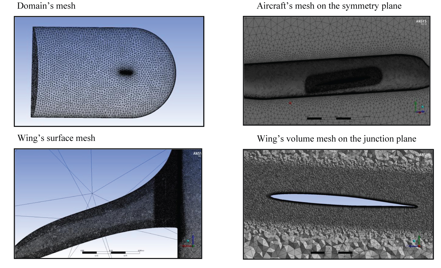
The resultant meshes are illustrated in Figure 5. Both the hybrid kind of the mesh, as well as the effect of implementing regions of higher grid's density is observable in that figure.

Grid-independency study

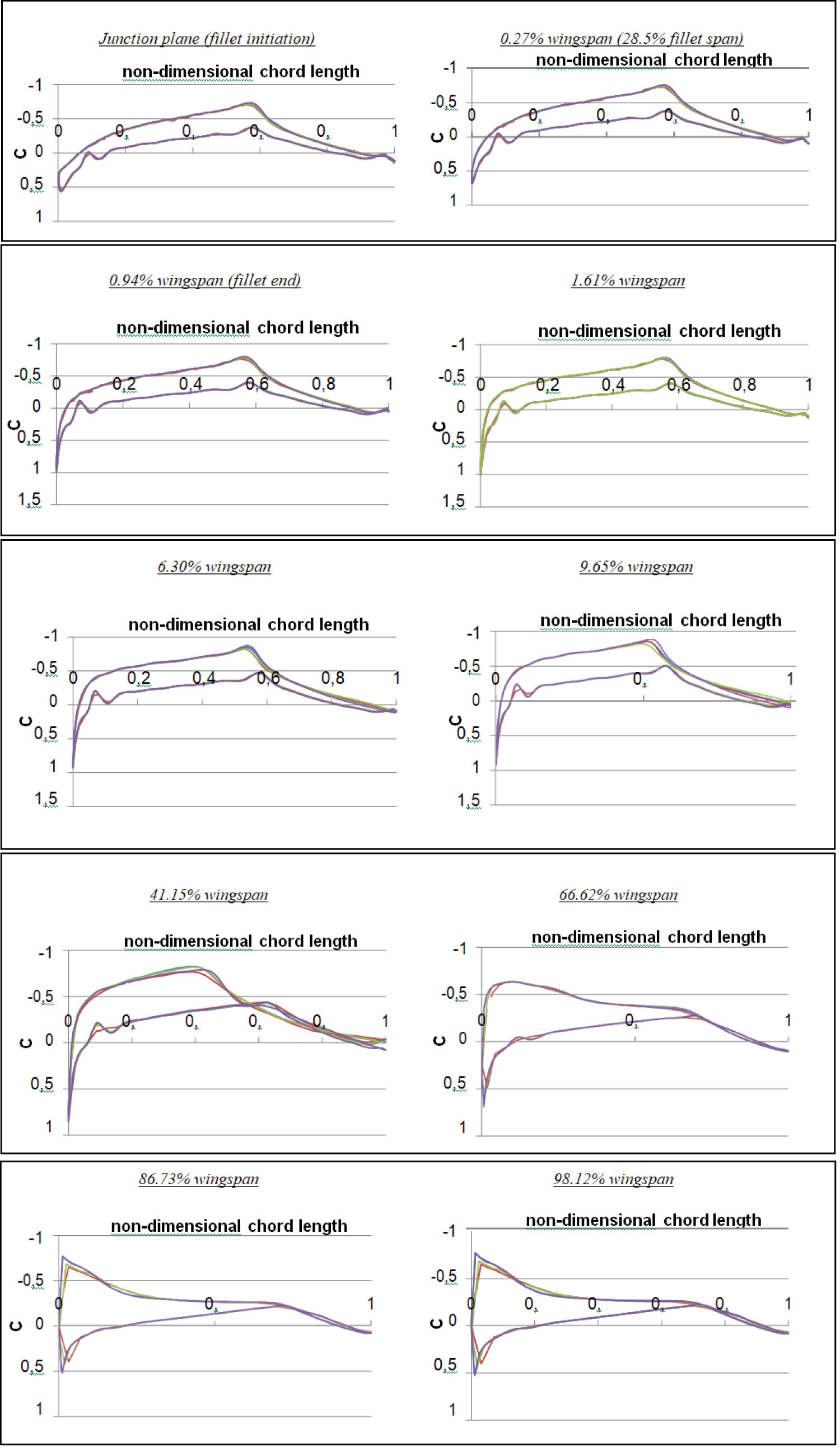
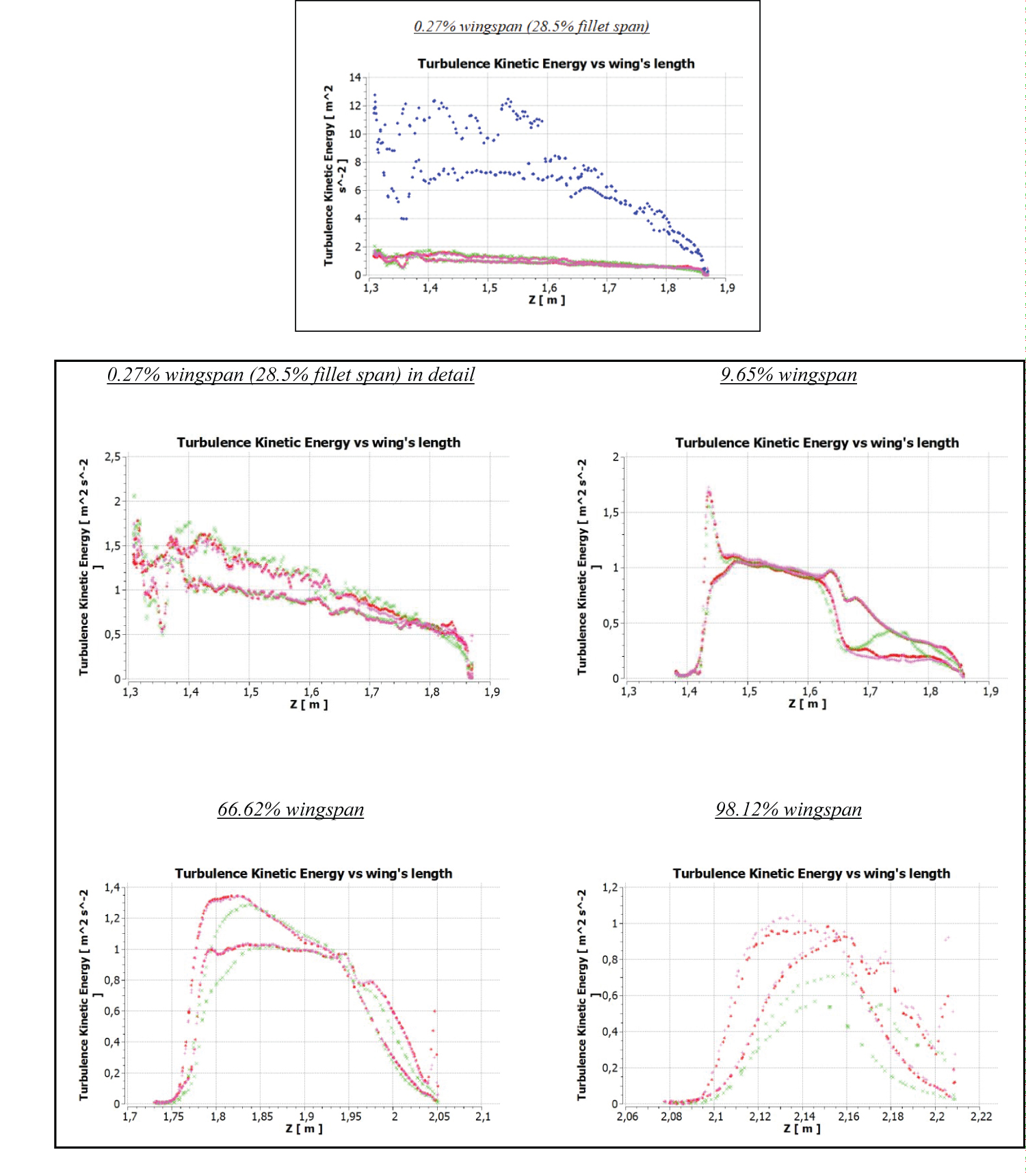
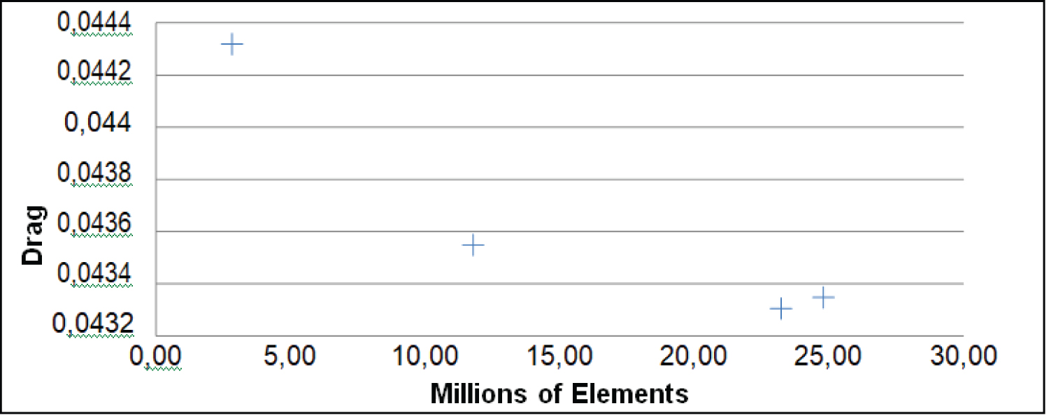
Four varieties of grid were implemented for each geometrical configuration, in order to obtain grid-independent results. The resulted meshes in our test cases were refined gradually, by refining the grid everywhere. Table 1 shows the selected grids and the number of elements that each grid consists of, in order the results for each configuration to be grid independent. For the sake of clarity, the dependence of the results on the grids used is presented in Figure 6 and Figure 7 that show the variations of pressure coefficient and turbulence kinetic energy distribution at the wall and the wall-adjacent cell centroid respectively, along the wingspan for four grids, as shown in Table 2, for the 3^rd configuration. Similar behavior is shown for all configurations, leading to the required number of elements as shown in Table 1. Additionally, as illustrated in Figure 8, grid independent study has been done for the drag coefficient internal parameter.

As it is shown in Figure 6, all meshes give similar outcomes, but for the discussion of the results we use the most accurate and fully grid independent one. Although inspection of Figure 6 suggests that the results for 2.4 million and 24.8 million elements are more or less similar, the reason the finer grids are needed is that, apart from the junction region, where the B.O.I is used, further outside this area the differences of the results is greater. Particularly, pressure coefficient distributions on the 9.65%, 41.15%, 86.73% and 98.12% of the wingspan, show that the proper grid selection is the "fine grid", since the "coarse grid" results show some variations compared with the results of the more detailed meshes, while the even "finer grid" does not lead to any further change to the results. So, despite the fact that the scope of this research work is to investigate the junction flow's characteristics, the grid independency for all the cases along the whole span is a determinant factor for accurate results and correct comparison of the aerodynamic effect of the junction modifications in all cases. Furthermore, for the verification of the grid independency, another significant parameter is considered in the present research work, which is the turbulence kinetic energy since it is strongly connected with the formed vortices characteristics. Under this consideration, Figure 7 shows that the "coarser grid" overestimates the turbulence kinetic energy even at the junction section, where a mesh refinement is applied via the B.O.I, making it an inappropriate choice, so it is not investigated further as a grid choice. At the same time, the 9.65%, 66.62% and 98.12% of the wingspan sections highlight that best choice is the selection of "fine grid", since "coarse grid" case shows some variation of turbulence kinetic energy, while the even "finer grid" does not result in further change. Lastly, for verification purposes an internal parameter is employed, the drag coefficient, which converges in the "fine grid" case, as shown in Figure 8, reaching the drag coefficient convergence less than half count (1 count = 0.0001). All in all, for the reasons stated above the chosen grid for the simulation conclusions is the "fine grid" case.

Similar behavior is shown for all configurations, leading to the required number of elements, as shown in Table 1.

Results and Discussion

Turbulence models

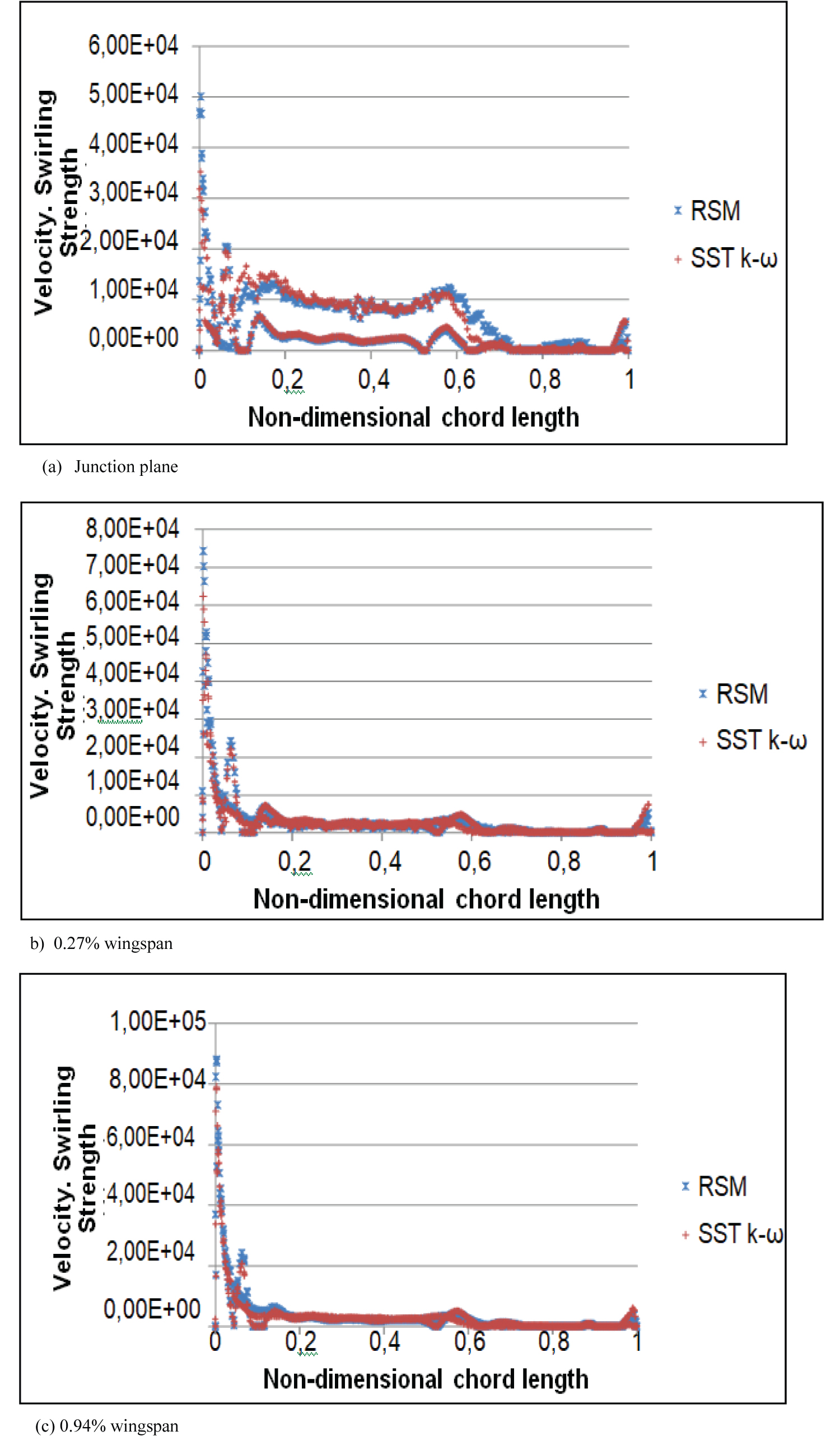
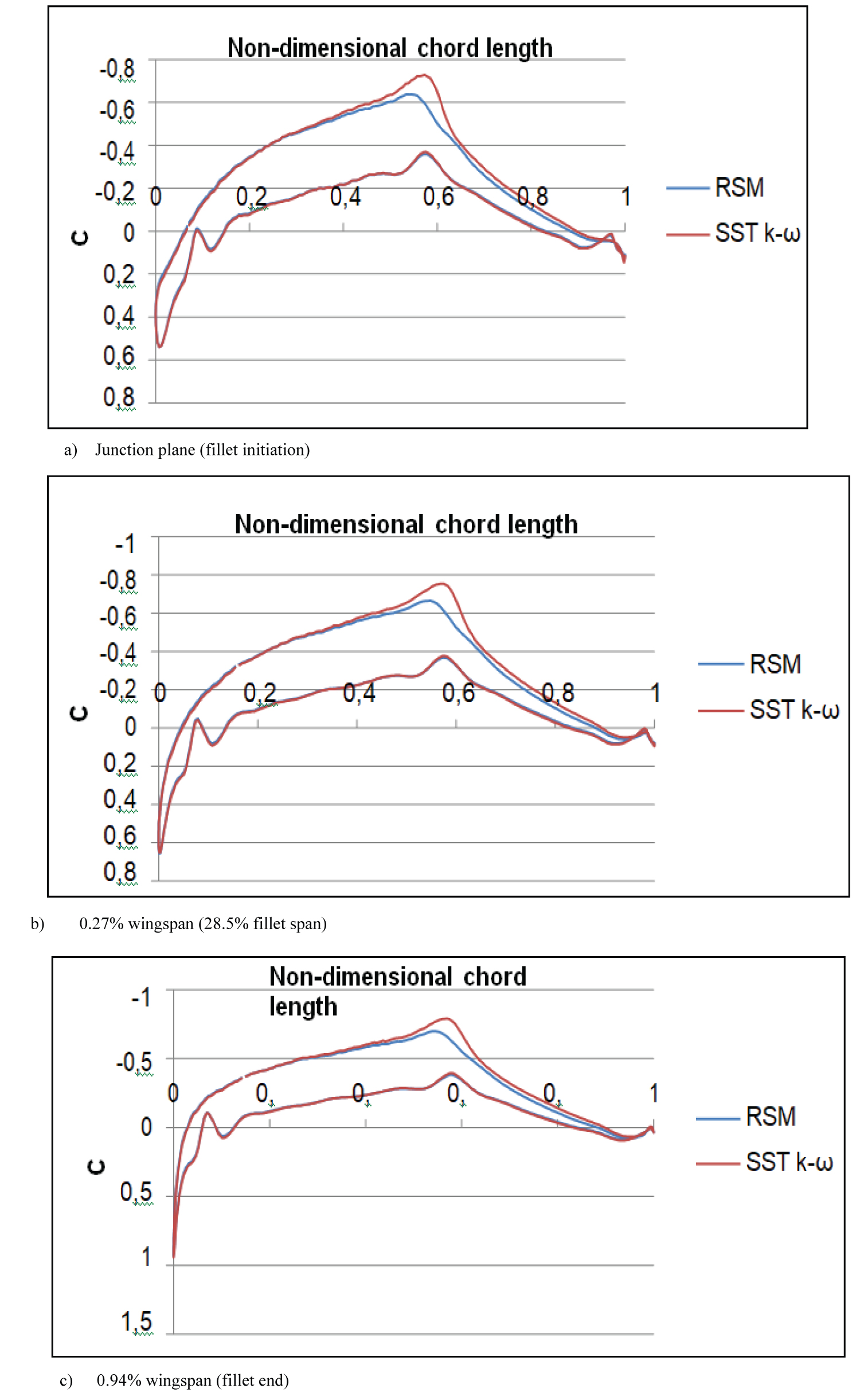
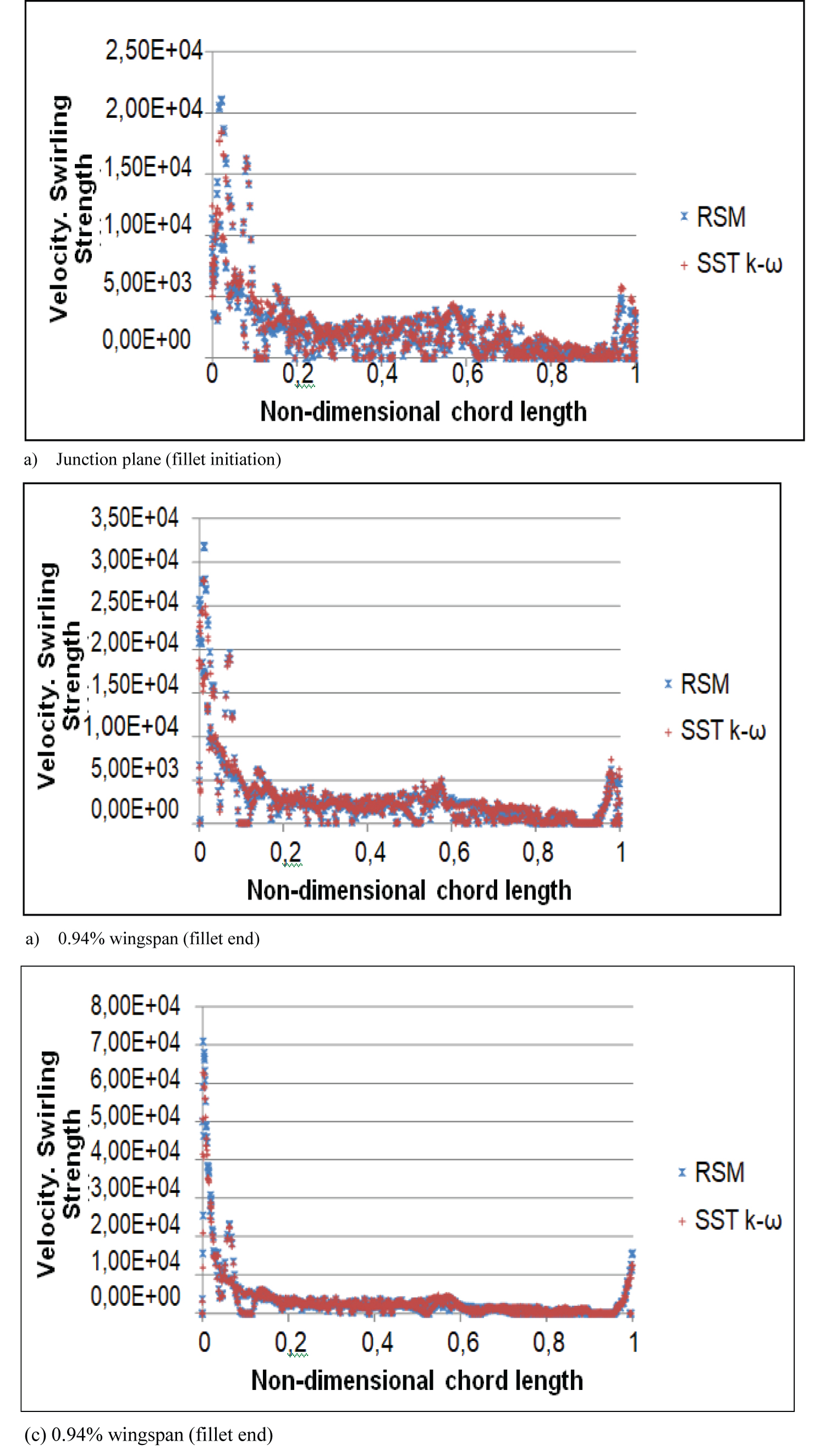
The turbulence models that have been used are the first-order closure modified SST k-ω model and the second- order RSM, as mentioned in section 2 above. The biggest differences observed between the predictions obtained by the RSM and by the modified SST k-ω models occur for the geometrical configuration 2. They concern the pressure- coefficient distribution along the junction chord sections downwind the 50% of the local chord, as illustrated in Figure 9. This results in slightly different prediction of the corner separation size between the modified SST k-ω model and the RSM. However, the variations concerning the swirling strength along the chord for the same case are limited and they are similarly predicted by both turbulence models, even for the most critical area that of the junction region, as illustrated in Figure 10. The velocity-swirling strength is defined as the imaginary part of the complex eigenvalues of the velocity gradient tensor and it describes the strength of the local swirling motion inside the vortex as well as the inner structure of the vortex and determines the vortices' local intensity characteristics. All the other sections have smaller differences and a typical example of the most critical area of the junction region is given in Figure 11 and Figure 12 for configuration 3, where the peak pressure coefficient seems to be their only difference. It should be mentioned that Apetrei, et al. [50] underline the SST k-ω superiority at transonic flows at low angles of incidence, under the spectrum of the more precise capturing of the wing's aerodynamic coefficients, while RSM tends to over predict the lift coefficient values and capture the shock waves location further downstream. Both of the Apetrei, et al. observations interpret the differences of the pressure coefficient distributions in Figure 9 and Figure 11, despite their similar results in general, indicating the SST k-ω model to be the proper one for assessing the aerodynamic improvements caused by the geometrical modifications. Furthermore, it should be underlined that both the first-order closure SST k-ω model, enhanced with rotation/curvature corrections and production limiters in order to limit the eddy viscosity in the junction region, and the second-order closure RSM model predict the same kind of vortical structures and give similar results. Additionally, as mentioned in section 2, the SST k-ω model modification should affect positively the more precise capturing of the junction flow, even at the corner separation cases. Therefore, the discussion of results and the design conclusions are presented for the modified SST k-ω model, because it is 7 times faster than the RSM to converge, since the latter solves seven transport equations rather than two (8 hours CPU time for the modified SST k-ω model versus 56 hours CPU time for the RSM model). This is of significant practical importance for the design engineer.

Aerodynamic results

The design modifications that took place have improved the junction flow regime in terms of the vortical structures characteristics, as it will be analyzed below. The improvement of the vortical structure status has contributed to the reduction of the drag force, which is translated in terms of aerodynamic efficiency in Table 3. Specifically, it has been achieved 17.20%, 23.06% and 57.28% improvement of the aerodynamic efficiency for the 1^st, 2^nd and 3^rd modifications, respectively, for that flight condition. Of course, the increased aerodynamic efficiency may also be a factor of other parameters; however, the junction flow characteristics affect certainly the aerodynamic efficiency of the integrated wing- fuselage junction design. After all, NASA Juncture studies [10-16] investigate junction flows to capture the corner separation, which will result in drag force reduction, highlighting the importance of the vortical structure characteristics at the junction region for the aerodynamic design of a wing-fuselage junction.

Vortices' analysis and topology

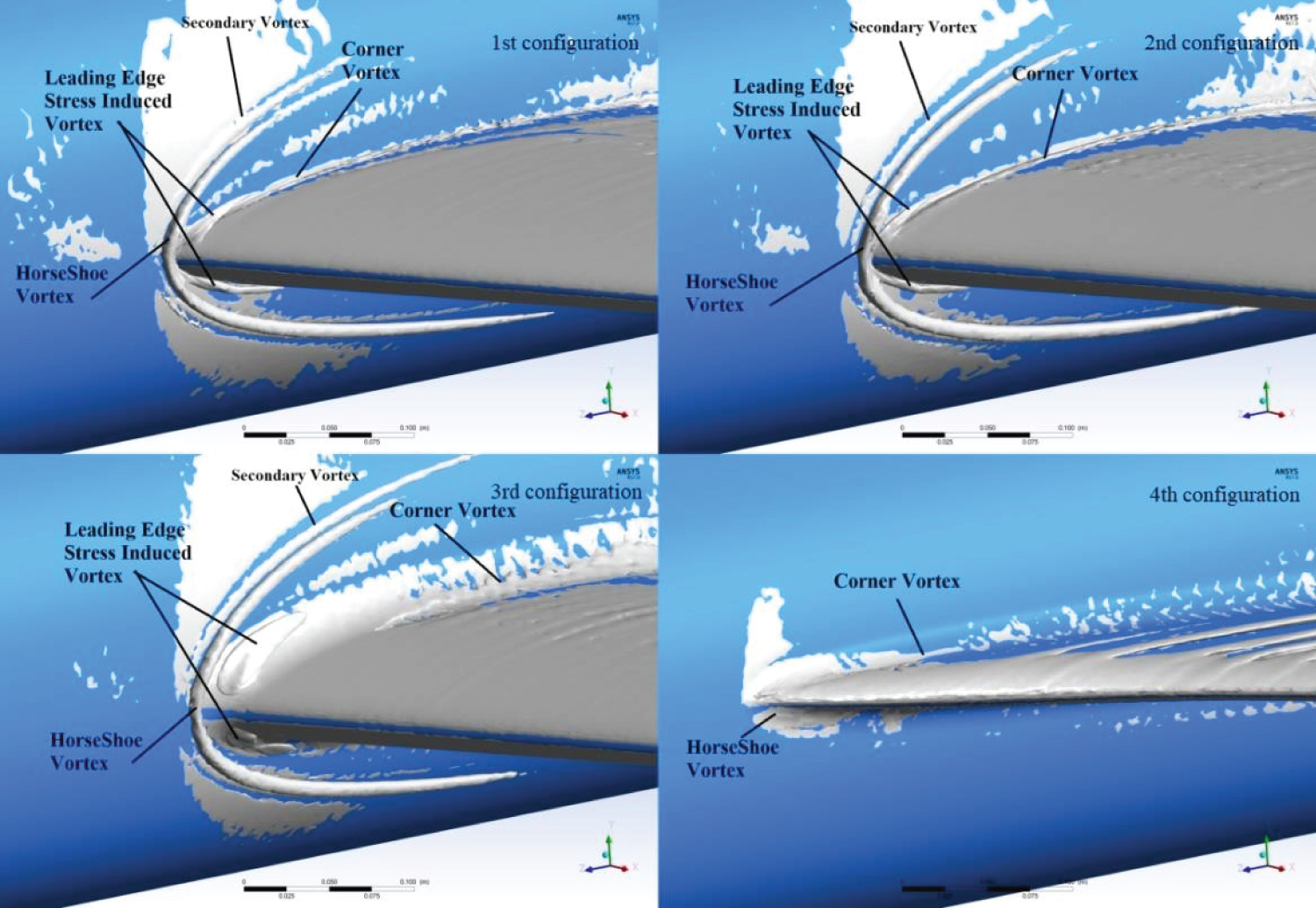
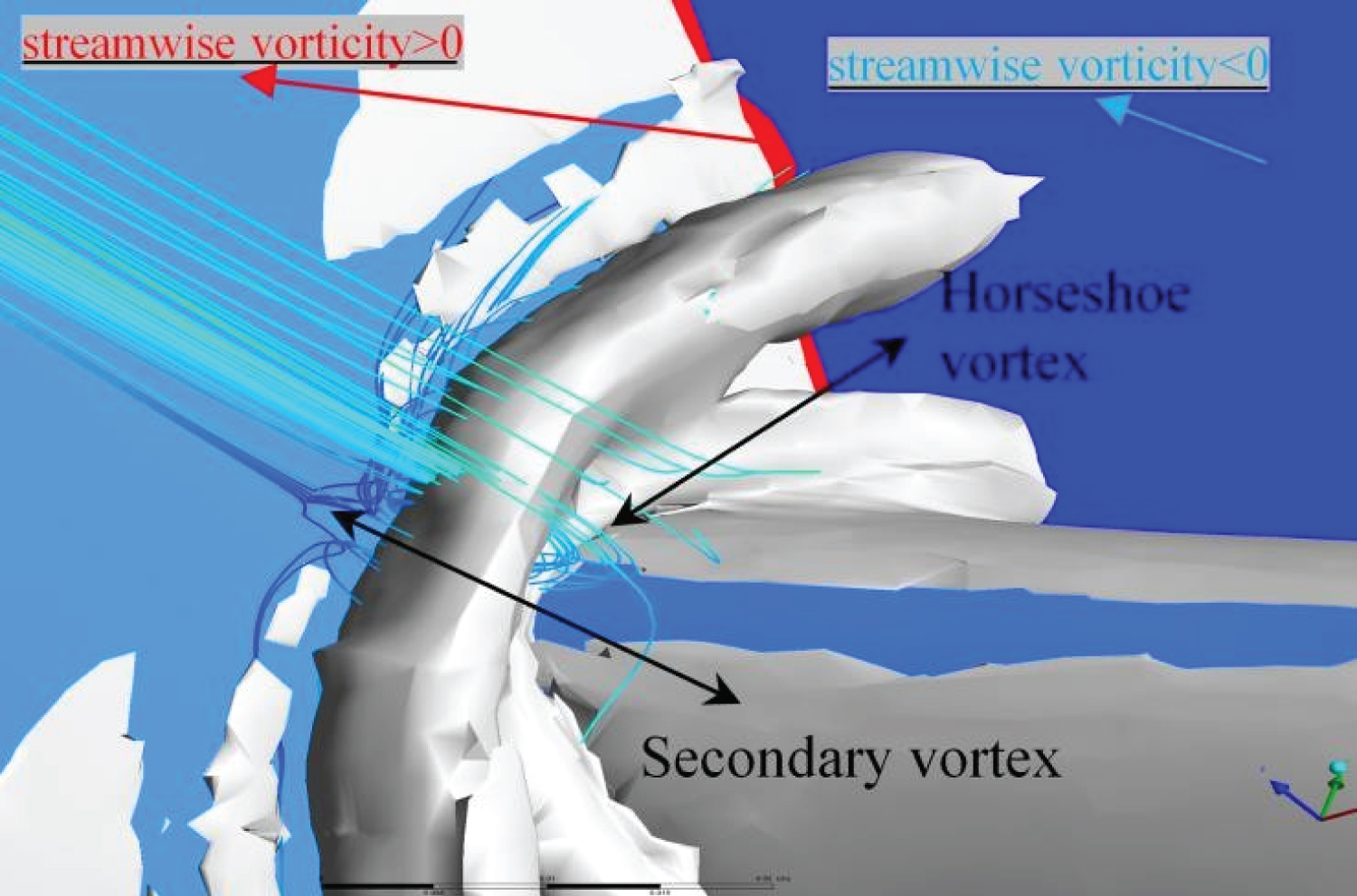
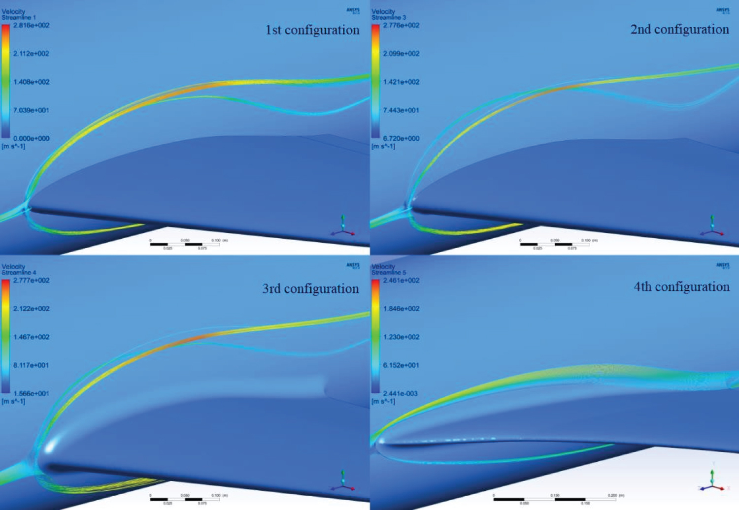
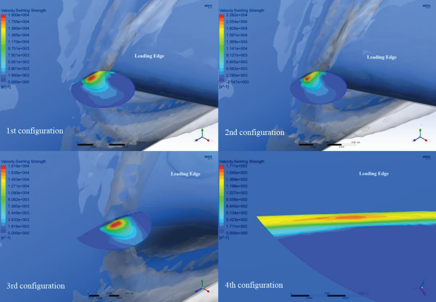
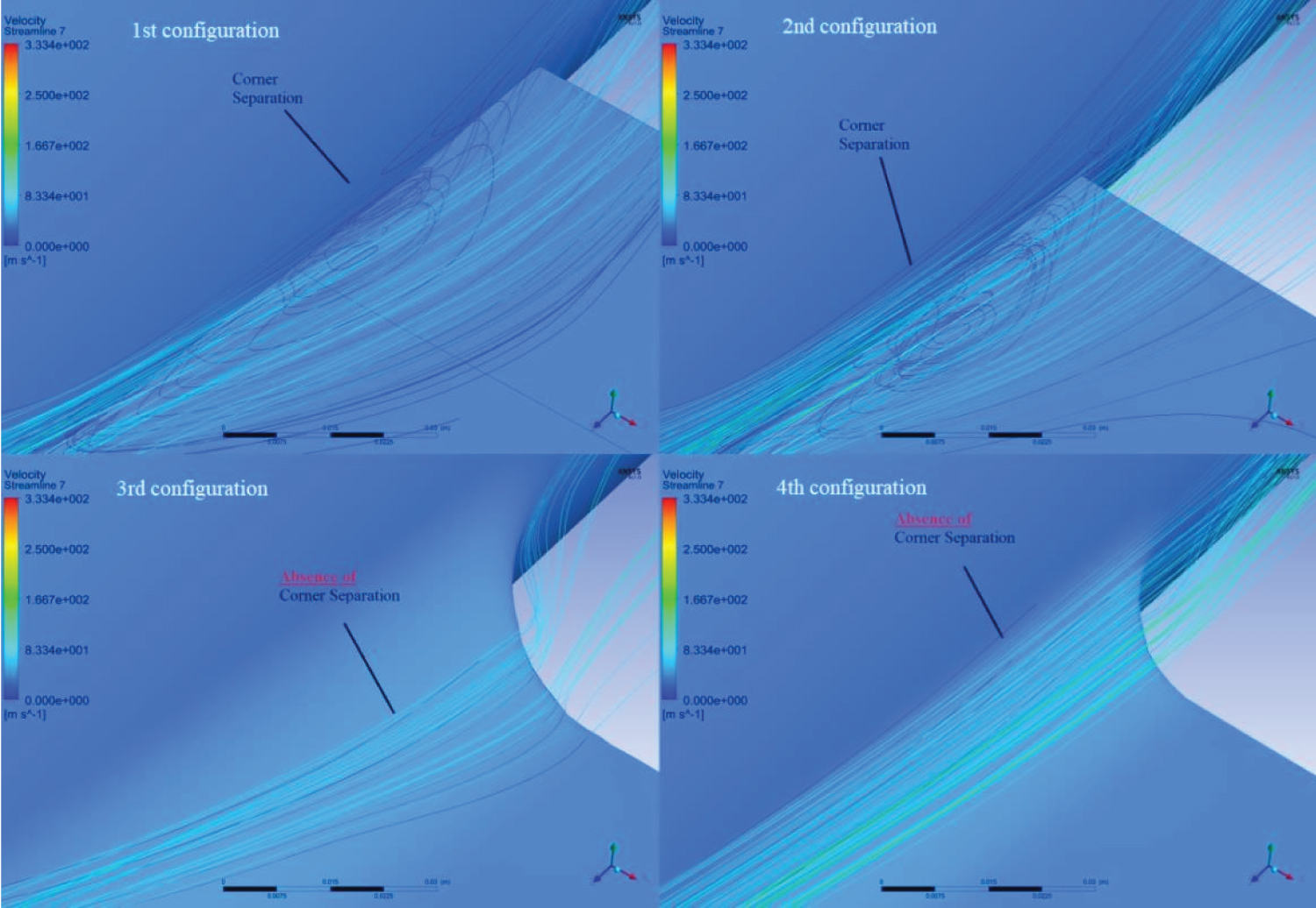
The numerical simulations showed that four types of vortices coexist at the tested junction flows. In order to visualize these vortices' structure and topology, the λ₂-criterion is employed. Figure 13 illustrates that the revealed structures are the horseshoe vortex, the secondary vortex, the corner vortex and the leading- edge stress- induced vortex. It is clear that all the four kinds of vortices are present at all configurations, except for the fourth configuration, where only the horseshoe and the corner vortices are formed. Some further observations are useful here:

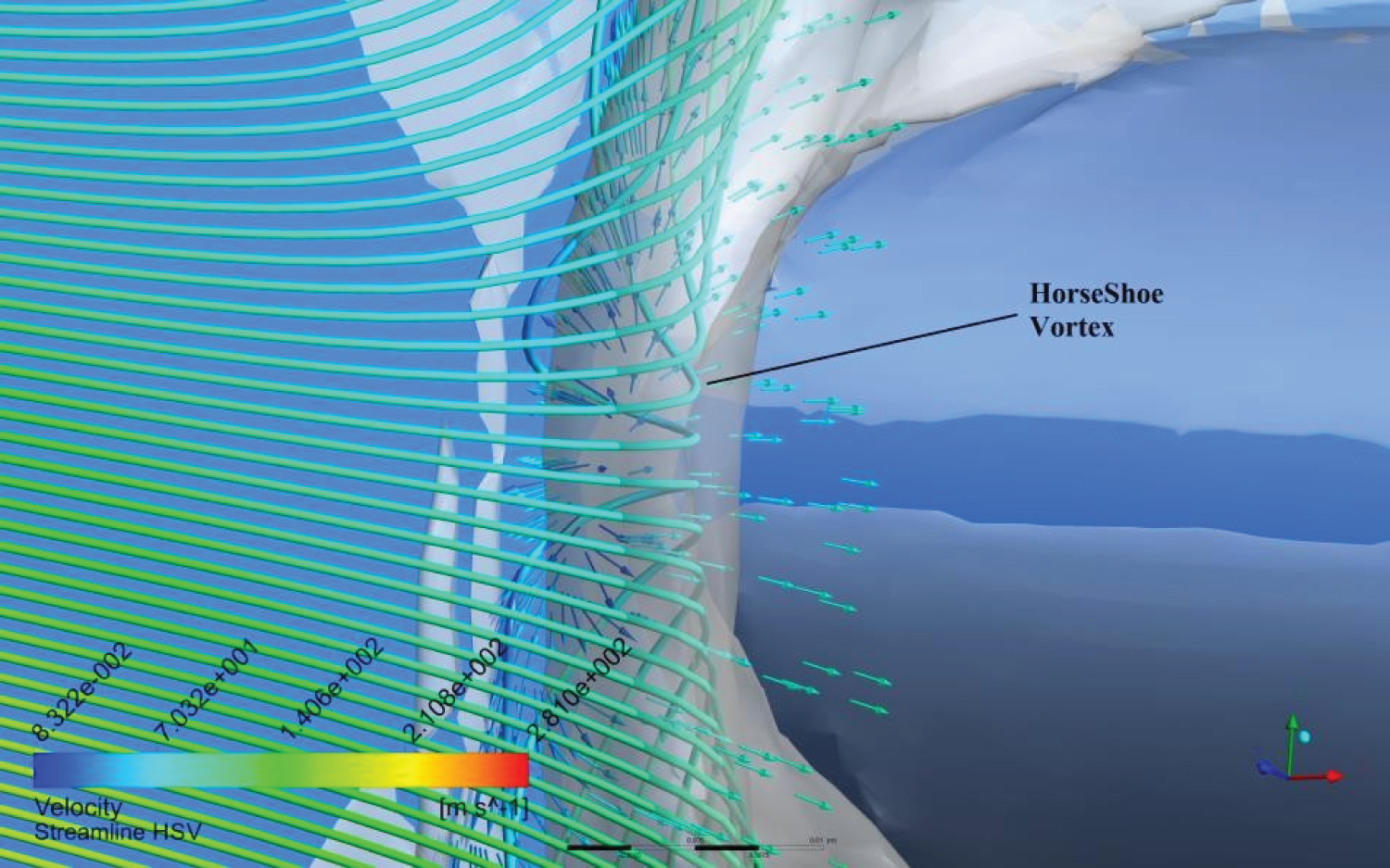
• The horseshoe vortex is the largest vortex of the junction flow and it is generated by the separation of the incident boundary layer (Figure 14), because of the adverse pressure gradient, which is generated because of the wing's presence. The horseshoe vortex, at all cases, is not attached to the fuselage surface. The formation of the horseshoe vortex is illustrated in Figure 15 and the adverse pressure gradient is illustrated in Figure 16.

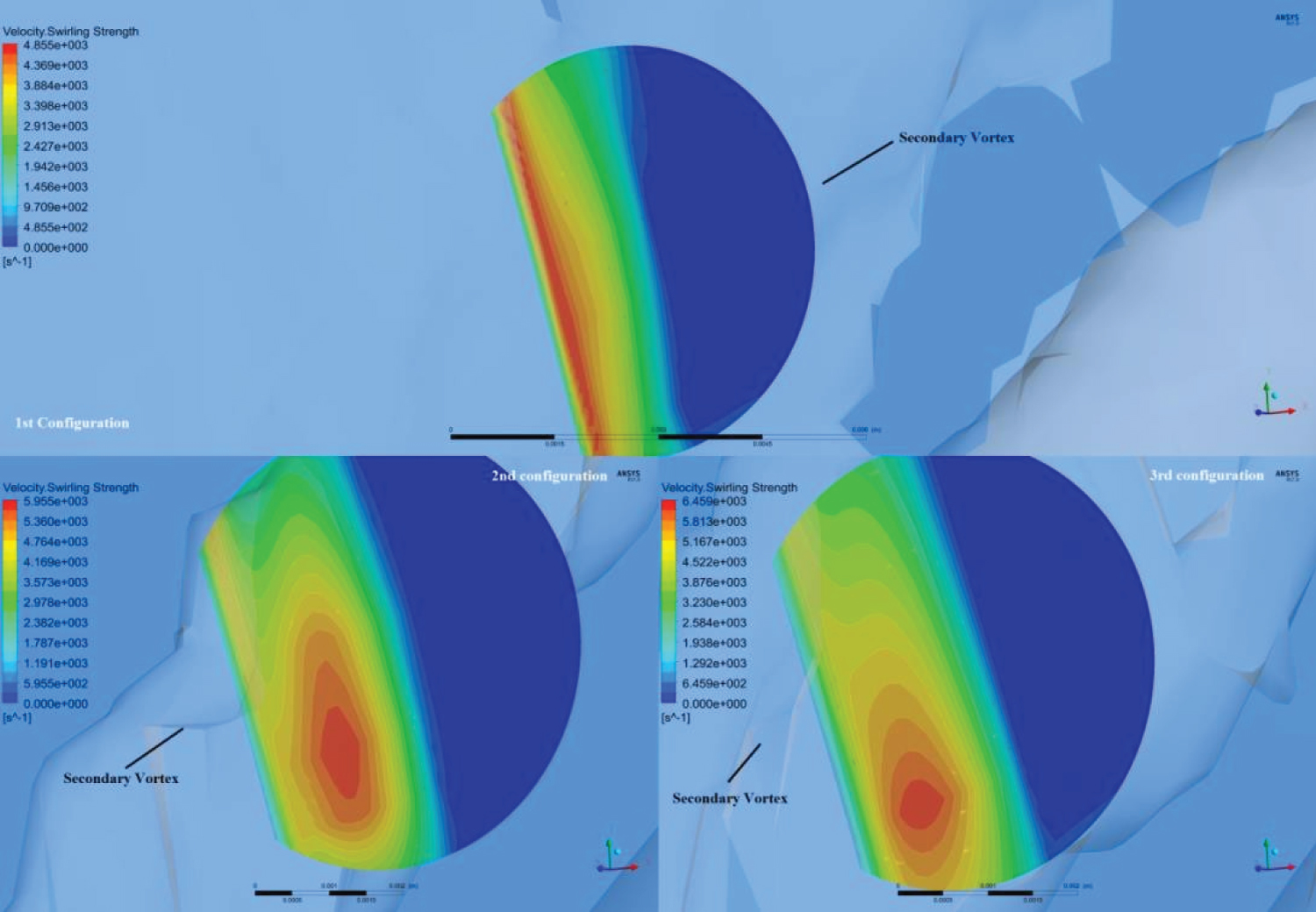
• The secondary vortex is another vortex structure, which is formed because of the impact of the incoming boundary layer with the adverse flow near the wing's leading edge. Contrary to the horseshoe vortex, the secondary vortex is developed very closely to the fuselage surface and it evolves along its curved surface. Figure 17 illustrates the formation and the slit of the secondary vortex from the flow. Figure 16 illustrates also a smaller region of adverse pressure gradient, which is connected to the presence of the secondary vortex.

• The corner vortex is another vortex structure, which is located at the wing-fuselage juncture. This vortex is generated at the wing's leading edge, it is transported along the juncture and it can interact with the probable corner separation.

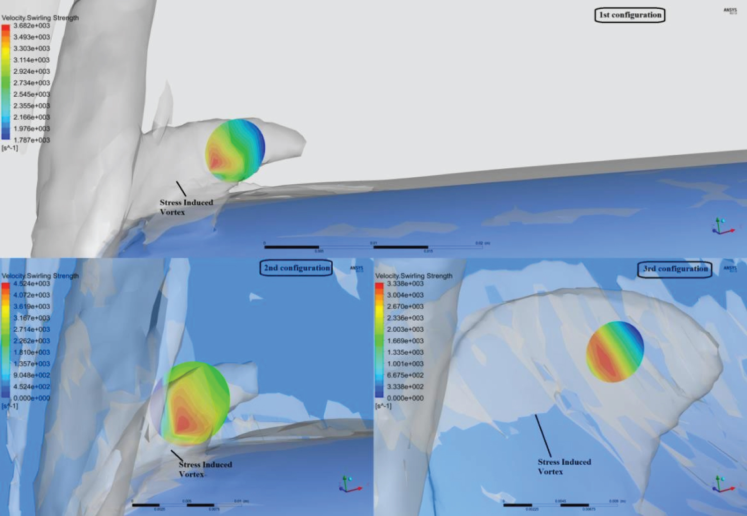
• The leading -edge stress- induced vortex is the last formed vortex structure, which is generated at the wing's leading edge by the primary stresses i.e. wv and wu gradients (z: longitudinal axis), whose magnitude is high because of the regions with high accelerations.

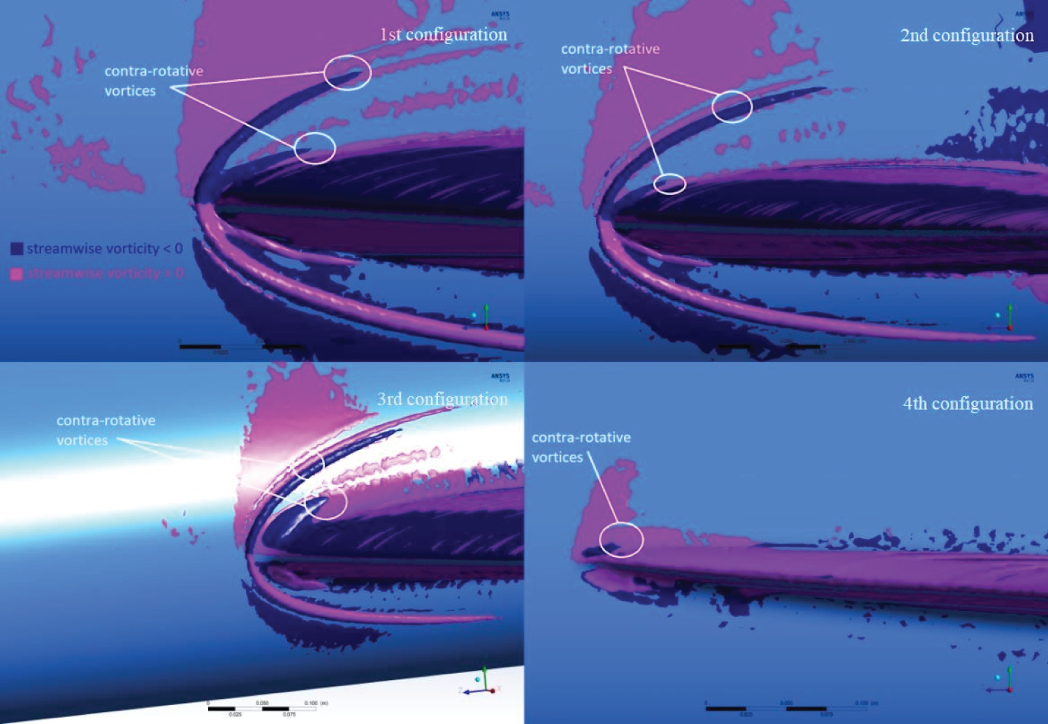
In Figure 18, it is seen that for all cases, the vortices rotate respectively in the same manner, therefore there is no secondary and leading -edge stress- induced vortex on the 4^th configuration. However, because in all configurations, they all appear in contra-rotative pairs, there is indirect evidence of the physical validity of the results. Particularly, the horseshoe vortex and the leading -edge stress- induced vortex are co-rotating vortices, in contrast with the secondary vortex and corner vortex, which are contra-rotating compared with the former vortices. The stream wise vorticity sign indicates the vortices direction of rotation.

Horseshoe vortex topology

To analyze the horseshoe vortex topology, firstly the B.F. and the M.D.F. should be defined. Specifically:

$$B.F.=\frac{1}{2}\frac{R_0}{X_T}\left(\frac{T}{S_T}+\frac{S_T}{X_T}\right)\text{ (17)}$$

Where T is the maximum thickness of the wing, XT the chord-wise location of T, ST the distance from the leading edge along the airfoil surface to the maximum thickness and R0 the leading-edge radius, as illustrated in Figure 19. The Bluntness Factor, which is computed from the airfoil's shape, indicates that round leading-edge shapes create stronger horseshoe vortices, as opposed to the sharp leading-edge shapes, as illustrated in Figure 20 [51].

and

$$M.D.F_X={\mathrm{Re}}_T\mathrm{Re}{\theta }_x={\left({\mathrm{Re}}_T\right)}^2\frac{{\theta }_x}{T}\text{ (18)}$$

Where,

$${\mathrm{Re}}_T=\frac{1}{2}\frac{UT}{v}\text{ (19)}$$

$${\mathrm{Re}}_{\theta x}=\frac{1}{2}\frac{U{\theta }_x}{v}\text{ (20)}$$

Where v is the fluid's kinematic viscosity, ReT is the Reynolds number based on the wing's thickness and Reθx is the Reynolds number based on the boundary layer momentum thickness at the location, where M.D.Fx is calculated.

For all the flow regimes, including the compressible conditions, the momentum thickness is calculated as follow:

$$\theta ={\displaystyle {\int }_0^{\infty }\frac{\rho \left(y\right)u}{{\rho }_{0}U}}\left(1-\frac{u}{U}\right)dy\cong {\displaystyle {\int }_0^{\delta }\frac{\rho \left(y\right)u}{{\rho }_{0}U}}\left(1-\frac{u}{U}\right)dy\text{ (21)}$$

Where ρ (y) is the fluid's local density, ρ₀ is the free stream density value, u is the local velocity, U is the free stream velocity and δ is the boundary layer thickness.

As mentioned in the introduction, the horseshoe vortex characteristics are mainly depended on the B.F. and M.D.F. values. Considering the M.D.F. values of the incoming boundary layer, this ranges from 1.09e+10 to 1.15e+10 for all the cases, at the z/c=-0.2 location (z: longitudinal direction). However, this study employed the M.D.F. calculations on the combined wing's and fuselage's boundary layers at the wing's root maximum thickness, which is crucial for understanding the horseshoe vortex legs behavior and topology, since the maximum thickness is a critical point where the axial velocity distortions determine the horseshoe vortex legs' evolution. Under this consideration, a high-level axial velocity distortion at the wing's root maximum thickness reveals the tendency of the horseshoe vortex legs to come closer to the wing's surface, and vice versa. At the same time, as the root's wing maximum thickness point is concerned, the calculation of the M.D.F. there gives a good view of the vortex evolution up to that point and inductively provides indications about its upwind regime and its strength. So, the following M.D.F. calculations are referred to the combination of wing's and fuselage's boundary layers at the wing's root maximum thickness.

The computed values of these factors are presented in Table 4. As shown in that table, the implementations of surface modifications had serious impact on the B.F. and M.D.F, since the different configurations present significant variability of their values. This variability interprets the different behavior of the horseshoe vortex in the junction flow.

The first aspect of the horseshoe vortex topology refers to its initiation point and its distance from the wing's leading edge. The second aspect of the horseshoe vortex topology is related with the way that it is developed along the junction. The last aspect is the distance of the horseshoe vortex legs from the wing's surface. Table 5 illustrates some useful horseshoe vortex characteristics for the whole analysis.

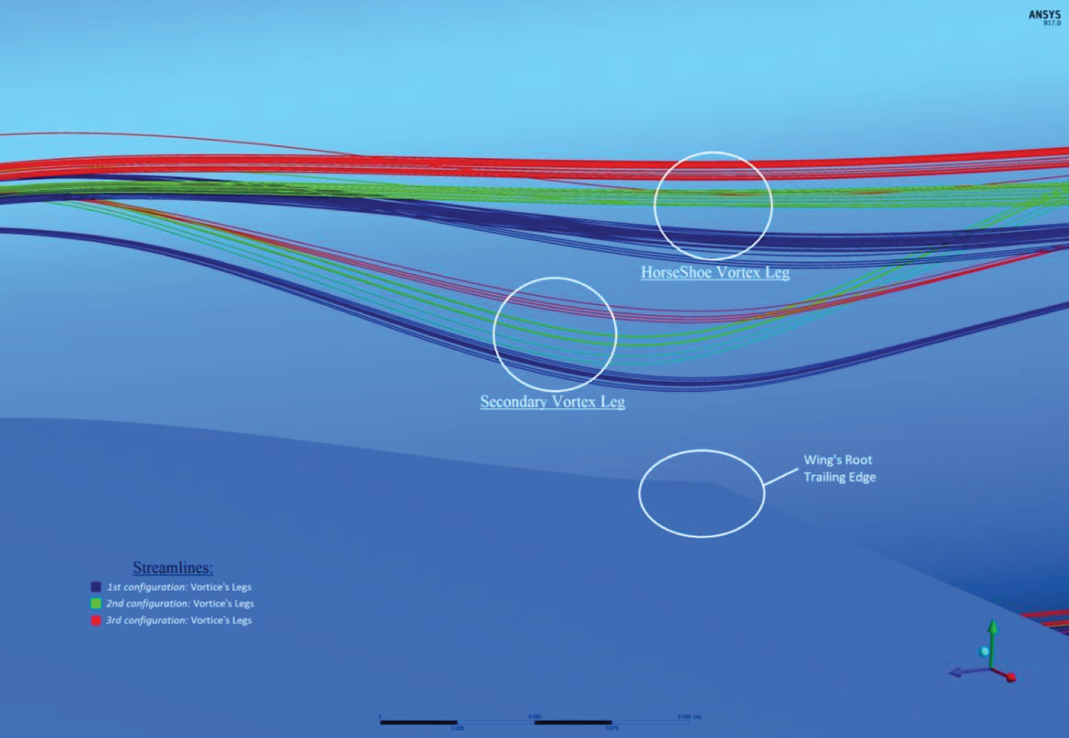
1^st modification: As far as the 1^st modification is concerned, the main, and critical for the flow, geometrical difference between the 1^st and the 2^nd configurations focuses on the sweep angle at the junction region. The 1^st configuration, at the junction region, has standard sweep angle (26.82°). On the other hand, the 2^nd configuration has smaller sweep angle, which is gradually getting smaller. Given that the 2^nd configuration has higher B.F. and that it has also a smaller sweep angle at the junction region, this combination results in and 24.63% increase of the distance between the initiation point of the vortex and the wing's leading edge. This is because both the high B.F. values and the small sweep angles cause the horseshoe vortex to be taken away from the wing's surface (Figure 21).

The results show that the horseshoe vortex develops along the junction in the same way for the two configurations. However, the horseshoe vortex legs of the 1^st configuration come closer to the wing's surface. The horseshoe vortex legs' behavior depends on the B.F., M.D.F, wing's sweep angle and the strength of the vortex. Therefore, despite the fact that the 1^st configuration has lower value of B.F., which produces a weaker vortex, the 36.57% increased value of M.D.F. and the larger sweep angle, make the vortex legs of the 1^st configuration, to come closer to the wing's surface.

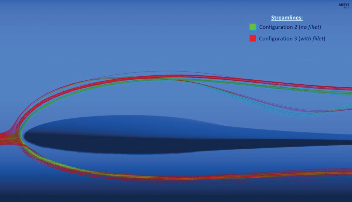
2^nd modification: The only geometrical modification between the 2^nd and 3^rd configurations is the constant radius fillet at the latter configuration. Therefore, the comparison between them underlines the effect of fillet surfaces on junction flows. Specifically, at the 3^rd configuration there is a remarkable increase in the B.F., as its value becomes 3.74 times higher than that of the 2^nd configuration. The B.F. increase is mainly due to the increase of the airfoil's active radius, because of the fillet inclusion. This increase has direct impact on the distance between the initiation point of the horseshoe vortex and the wing's leading edge, which grows by 71.60% relatively to the 2^nd configuration (Figure 22).

At the 3^rd configuration, the horseshoe vortex is pushed away from the wing's surface, while it is developed along the junction, as it is illustrated in Figure 23. Concerning the legs of the horseshoe vortex, the fillet configuration leads to legs that are more distant from the wing's surface. In this case, the higher values of B.F. and M.D.F. of the 3^rd configuration seem not to be the dominant criteria to interpret the horseshoe vortex legs' behavior. This is because the longer distance between the initiation point of the horseshoe vortex and the wing's leading edge, where the vortex initiates, and the weaker vortex seem to be the more crucial factors for the junction flow formation Figure 24.

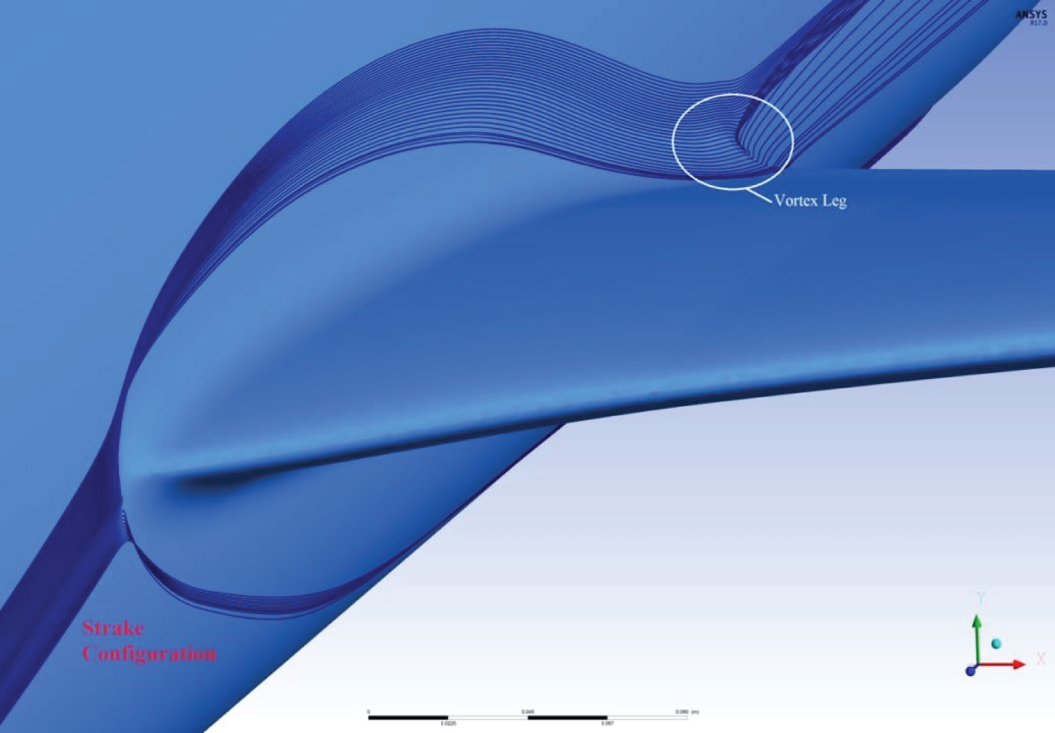
3^rd modification: The last modification addresses the strake effect on junction flows. It is noted that the 4^th configuration includes the fillet surface, in order to isolate and study the strake effect, when the 3^rd and 4^th configurations are compared. Because of the strake inclusion, there are differences in the sweep angle close to the junction region. Specifically, the 3^rd configuration, in the area where the junction flow takes place, has smaller sweep angle, which is gradually getting smaller (26.21°-22.69°) relatively to the 4^th configuration, whose sweep angle is gradually getting larger (56.07°-66.11°). Furthermore, the strake configuration has a sharper leading edge because of its airfoil.

Combining the larger sweep angle and the 38.09% lower B.F. value of the 4^th configuration, results in an important decrease of the distance between the initiation point of the horseshoe vortex and the wing's leading edge. Therefore, the insertion of the strake surface causes the horseshoe vortex to wrap around the wing and contributes to its elimination.

Regarding the development of the horseshoe vortex, its streamlines come much closer to the wing's surface and its legs come in contact with the wing's trailing edge (Figure 25). The 2.44 times higher M.D.F. value of the 4^th configuration and the larger sweep angle are the dominant factors, which explain the horseshoe vortex legs' behavior.

Horseshoe vortex strength and size

1^st modification: The 1^st and the 2^nd configuration have similar sized horseshoe vortices, but the 1^st configuration's vortex is slightly smaller. However, their core shape and strength are different, which affect their spatial diffusion, as shown in Figure 26. The horseshoe vortex of the 2^nd configuration has higher swirling strength, as it has higher B.F. value, smaller sweep angle and more intense adverse pressure gradient faced by the incoming boundary layer, which prevail over its lower M.D.F. value. It is clarified that the swirling strength in the current study is defined the imaginary part of complex eigenvalues of velocity gradient tensor. It is positive if and only if the discriminant is positive and its value represents the strength of swirling motion around local centers [40].

2^nd modification: The computational results of the 2^nd modification show that the fillet geometry introduction causes larger sized horseshoe vortex. It is observed that the fillet introduction causes the core shape adaption to the local fillet curvature, where the vortex is generated (Figure 26). In addition, the horseshoe vortex of the 2^nd configuration has higher swirling strength comparing with the 3^rd configuration. The more intense adverse pressure gradient faced by the incoming boundary layer of the 2^nd configuration is proved to be more dominant criterion of higher swirling strength vortex, than the B.F. and the M.D.F., which have higher values at the 3^rd configuration.

3^rd modification: The 3^rd modification introduces the strake effect on junction flows. The computational results of the 4^th configuration show that the strake eliminates and weakens the horseshoe vortex. Specifically, Figure 26 illustrates that the strake configuration produces a much smaller sized horseshoe vortex compared with the 3^rd configuration. The fact that the 4^th configuration contains fillet geometry confirms that the core shape is adapted to the local fillet curvature, as happened with the 2^nd modification (Figure 26). The lower B.F. values, the larger sweep angle and the weaker adverse pressure gradient faced by the incoming boundary layer are the main factors, which result in the presence of weaker horseshoe vortex at the 4^th configuration.

Secondary vortex

The secondary vortex is a lower strength vortex, which qualitively follows the horseshoe streamline pattern, but it is counter-rotating to the latter vortex. This kind of vortex is present only at the first three configurations.

The higher maximum swirling strength of the secondary vortex takes place at the 3^rd configuration, while the lower maximum swirling strength is shown at the 1^st configuration (Figure 27). Except their swirling strengths, the secondary vortices have also different core shapes, which are due to their different way of evolution in the flow. The swirling strength of the secondary vortex seems to be directly related to its legs' topology, since the higher the swirling strength, the closer the proximity of the secondary vortex legs to the wing's surface. Interesting to observe that, as illustrated in Figure 23, the results for all the configurations show that the secondary vortex legs approach closer the wing compared with the horseshoe vortex legs.

Leading- edge stress-induced vortex

The leading- edge stress- induced vortex is a smaller vortex structure with lower swirling strength, which is present at the first three configurations. The higher maximum swirling strength of the leading- edge stress- induced vortex takes place on the 2^nd configuration, while the lower maximum swirling strength appears on the 3^rd configuration (Figure 28).

Responsible for the leading- edge stress- induced vortex shape is the fillet effect (configuration 3), since, as illustrated in Figure 14, the fillet introduction causes a longer vortex, which adapts its shape to the local fillet curvature. Furthermore, the fillet affects the vortex swirling strength, causing a small drop of its values, as illustrated in Figure 28 for the 2^nd modification (comparison of 2^nd and 3^rd configurations).

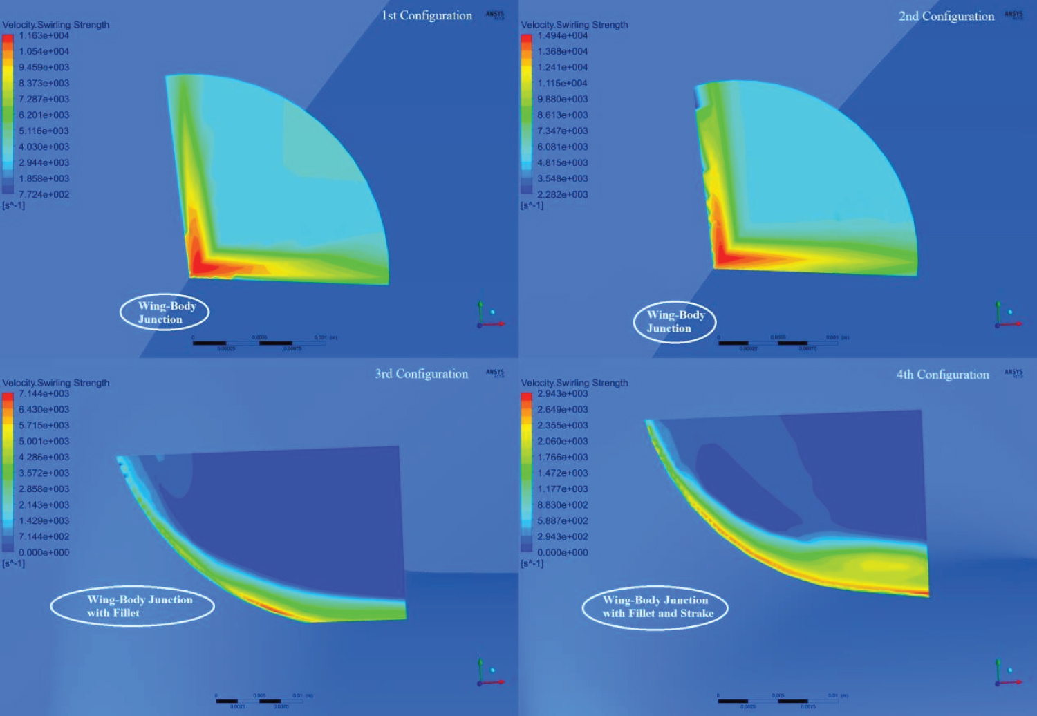
Corner vortex

According to the "λ₂- criterion", the last formed vortex structure is the corner vortex. It is noticed that the 1^st and the 2^nd configurations, whose wing-fuselage connections form a sharp corner, create stronger corner vortices, compared with the last two configurations (Figure 29). Specifically, at the 3^rd and 4^th configurations, where the junction connection is smoothed out by fillet and strake, respectively, it is shown that these types of geometrical modifications weaken the swirling strength of the corner vortex. The 2^nd modification is proved to reduce by 52.18% the vortex swirling strength and the 3^rd modification has reduced it further by 58.81% (comparing the 3^rd with the 4^th configurations). As a conclusion, the present study shows that the introduction of the fillet and strake can reduce the magnitude of the corner -vortex swirling strength by 75-80%, as compared to the sharp edge junction connections (1^st and 2^nd configuration).

Corner separation

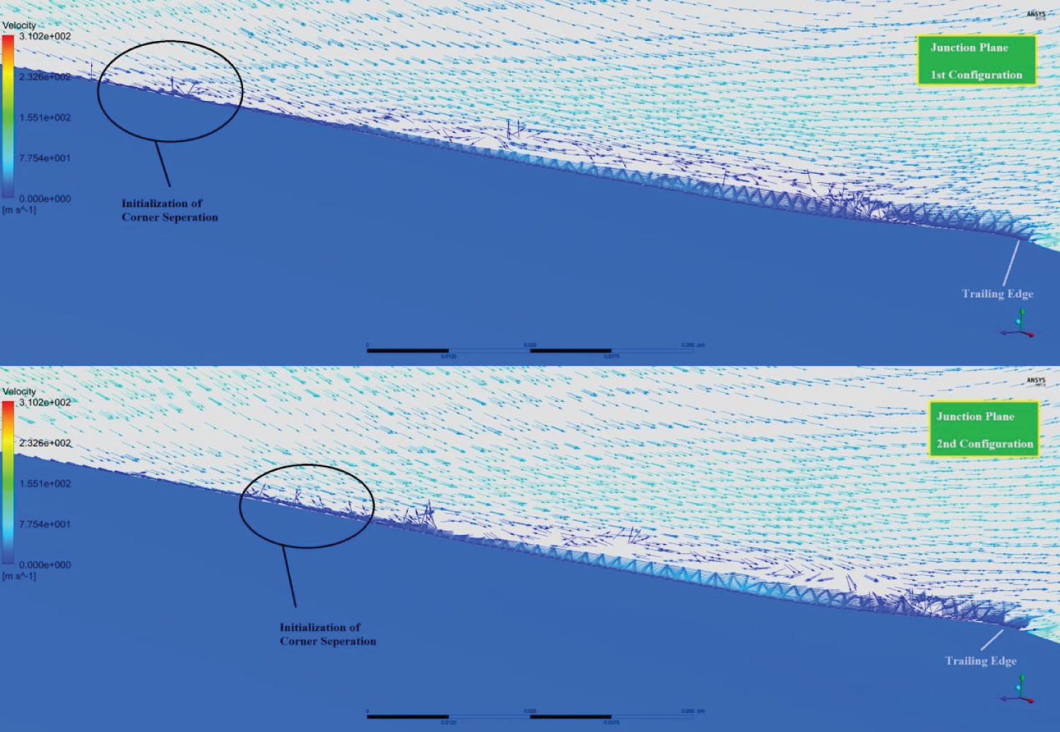
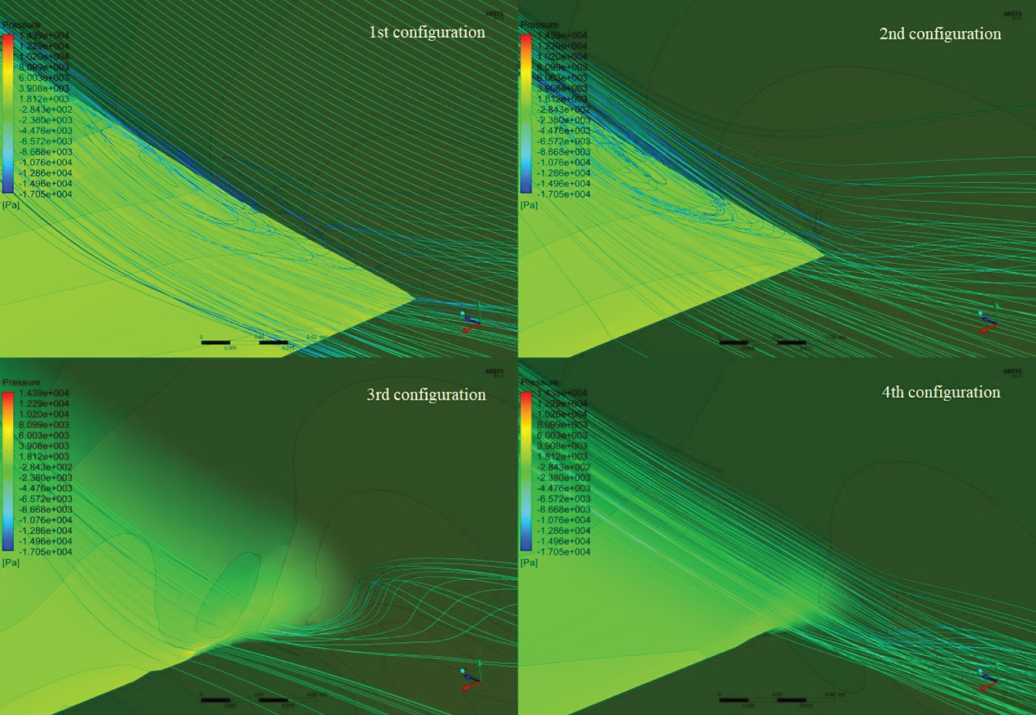
As illustrated in Figure 30, the corner separation takes place only in the 1^st and 2^nd configurations. Figure 31 shows that the corner separation initiates earlier in the 1^st configuration. From these computational results, it is obvious that the fillet and the strake geometries prevent the corner separation by smoothing the corner flow at the wing-fuselage connection.

The presence of the corner separation in the first two configurations is explained by the pressure increase at the wing's root trailing edge, which is not observed when the fillet and strake geometries are imported (Figure 32). In addition, at the first two configurations, the corner vortex is stronger because of their sharp edge junction connection, which means that the fuselage and wing's boundary layers strongly interact. This has as a result, the tendency of forming corner separation.

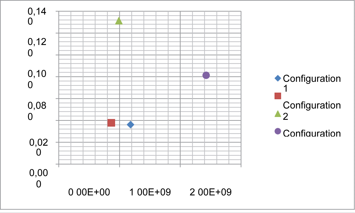
Results exports according to the B.F. and M.D.F. diagram

As the majority of studies report the dominance of B.F. and M.D.F. in the junction flow formation, it is interesting to mention the previews studies' combination of B.F. and M.D.F. values. The studies considered in this paper are using different types of turbulence modelling and some of them present experimental results. In Table 6, some of the preview studies' data and their B.F. and M.D.F. combinations [4] are summarized. It is worth mentioning that the current study approaches an unexplored area of M.D.F. and B.F. combinations, since the M.D.F. values of the incoming boundary layers range from 1.09e+10 to 1.15e+10, when the previous ones focus on a M.D.F. range from 7e+8 to 1.33e+9.

However, using the M.D.F. evaluation on the combined wing's and fuselage's boundary layers at the wing's root maximum thickness as proposed in this study, Figure 33 presents, in exponential scale, the area where this study lies among the M.D.F. and B.F. diagram, according to Table 4. It is shown that the choice of wings with high values of these two factors reduces the possibility of corner separation formation. Additionally, the effect of the 2^nd modification in terms of the spectrum of the B.F. and M.D.F. diagram should be highlighted. Specifically, the implementation of the 2^nd modification, by applying the fillet geometry, causes the rise of the corresponding point in the diagram.

This happens because of the root airfoil's active radius increase, which led to the smoothing of the junction flow and the existence of an area of no corner separation. Furthermore, the 3^rd modification was also effective, by implementing the strake. It led to a B.F. and M.D.F. combination, which contributed to no corner separation, helped to eliminate the secondary and leading- edge stress- induced vortices and greatly weakened the horseshoe vortex's swirling strength, all of which increased the aircraft's aerodynamic efficiency.

Comparison with current literature and experiments

The strake effect finds common ground with the DLR-F6 project, when a horn was entered into the wing configuration [81]. This NASA's horn geometry introduction had a similar function with that of the present study's strake, since it is considered as an extension between fuselage and wing at the leading edge, whose purpose is to mitigate the size and the strength of the horseshoe vortex. Both CFD and experimental results of the DLR-F6 project, showed that the horn has brought the horseshoe vortex initiation point closer to the wing's leading edge, while it produced a smaller leading edge horseshoe vortex, as shown in Figure 34 and Figure 35, exactly as the strake configuration case of the present study. This common finding highlights the influence of these types of geometries on the vortex structures and their topology in junction flows.

The strake influence in the junction flow of this study shows also similar and consistent results with the Devenport, et al. [60] study, which showed that the strake in their idealized appendage-body junction modified the flow characteristics in a desirable way, by reducing the adverse pressure gradient and by eliminating the horseshoe vortex.

As far as the fillet effect is concerned, the results of implementing the 2^nd modification in the present study are in agreement with Devenport and Simpson [82], since both studies indicate that the insertion of constant- radius fillet at the wing-body junctions, increases the size of the horseshoe vortex and displaces it away from the wing surface, because of the increased effective radius of the nose of the wing at the junction region. Nevertheless, there is a difference between these two studies in that Devenport and Simpson's results [82] indicate that the fillet introduction causes an increase in the horseshoe vortex strength, which is not the case with the present results. It should be mentioned in this context that the existing literature and reported experiments refer to cases with different Reynolds numbers and flow regimes to the present cases. However, the qualitative comparison is still important in order to deduce useful conclusions about the junction flow behavior.

Conclusions and Suggestions for Future Work

The present work has approached an unexplored area of high M.D.F. values of the incoming boundary layer (1.09e+10 - 1.15e+10), which an area of interest is referred to the modern literature as suggestion for future work. It is proposed an alternative use of M.D.F. on the combined wing and fuselage's boundary layers, at the wing's root maximum thickness that has been proved to predict successfully the horseshoe vortex legs behavior, as far as their evolution and their proximity to the wing's surface are considered. The results prove that to investigate the M.D.F. at the maximum thickness is essential, since the maximum thickness is a critical point where the axial velocity distortions determine the horseshoe vortex legs' evolution and the results obtains suggest that this is an additional parameter that should be considered in future junction flows studies.

A more extended view of junction flow vortex structures interaction is pursued in the current study and how this varies with specific geometry modifications. Despite the dominance of the horseshoe vortex that is reported in the literature, it has been shown that all the formed vortices interact with each other and that they can, with specific surface modifications, improve the junction flow characteristics. Specifically, according to the results, introducing fillet geometries to avoid the sharp junction edges and so the strong interaction of the fuselage and the wing's boundary layer, tends to eliminate the corner separation occurrence by reducing the corner vortices' strength by 75-80%. Fillet is also proved to be strongly connected with the leading- edge stress- induced vortex size and shape, and the horseshoe vortex core shape adapts to the local fillet curvature, affecting its spatial diffusion. Additionally, the local increase of the blended wing sweep angle parameter at the junction region delays the corner separation formation. It should be mentioned that all the conclusions about the corner separation presence, predicted by computational simulations, need further validation by wind tunnel experiments. Nevertheless, since the simulation has been also carried out with a second-order-closure turbulence model and the same turbulence model has been used in all cases, and has also been compared with other similar simulations existing in the literature, the authors are confident that, in a relative design manner, the design modifications that took place in the present research improved in a comparative sense the corner separation flow features.

A detailed analysis of the horseshoe vortex in all the configurations has taken place, under the aspects of its onset distance in relation to the wing's leading edge, its legs topology in relation to the wing's trailing edge surface and its swirling strength, and they all proved to be interdependent. This means that in the present work many more parameters have been taken into account than it is normally the case in the existing literature. The variety of the configurations studied, gave the authors the opportunity to export useful conclusions, since in real wing-fuselage junctions, parameters that do not exert impact in the same way coexist and so some parameters prevail over others. The exported conclusions support that, despite the B.F. and M.D.F. dominance on the horseshoe vortex formation, as reported in the modern literature and confirmed in the current study, the horseshoe vortex onset topology, its swirling strength, the local sweep at the wing's root region and the adverse pressure gradient upwind the wing's leading edge are parameters that should also be investigated, when junction flows are studied. Specifically, the high B.F. values and the small local sweep angles at the wing's root region proved to be connected with longer distances between the wing's leading edge and the horseshoe vortex initiation point. Additionally, the high B.F. and M.D.F. values, the large local sweep angles at the wing's root region, the short onset distances in relation with the wing's leading edge and the strong horseshoe vortices proved to be directly connected with the horseshoe vortex legs' proximity to the wing's trailing edge surface. This is a conclusion that also affects the corner separation regions, since the horseshoe vortices' legs bring higher momentum fluid in the boundary layer, when they penetrate the wing's boundary layer, resulting in corner separation elimination. Simultaneously existing higher B.F. and M.D.F. values, more intense adverse pressure gradient and smaller local sweep angles at the wing's root region lead to a stronger horseshoe vortex, and vice versa. Among the above parameters, the strongest one that tends to affect more the horseshoe vortex behavior appears to be the resulting adverse pressure gradient.

The junction design modifications' contribution is obvious through the analysis and the results, since each modification resulted in better flow regime of the junction region. The most promising design modification seemed to be the last configuration, where the fillet and the strake effects were combined. This configuration provides a more streamlined and efficient junction surface by eliminating the secondary vortex, the leading- edge stress- induced vortex and the corner separation and weakening the horseshoe and the corner vortices' swirling strength by an order of magnitude (Figure 26 and Figure 29), compared with the reference configuration. The better vortical structure status and flow management in the junction region resulted in reduced drag force, which is translated in terms of aerodynamic efficiency improvement.

Data Availability

The data that support the findings of this study are available from the corresponding author upon reasonable request.

References

1. Bradshaw P (1987) Turbulent secondary flows. Annual review of fluid mechanics. 19: 53-74.
2. Apsley D, Leschziner M (2001) Investigation of advanced turbulence models for flow in generic wing-body junction. Flow Turbulence and Combustion 67: 25-55.
3. Fleming J, Simpson R, Devenport W (1991) An experimental study of turbulent wing-body junction and wake flow. Tech rep Virginia Polytechnic Institute and State University, Aerospace and Ocean Department.
4. Gand F, Deck S, Brunet V, et al. (2010) Flow dynamics past a simplified wing body junction. Physics of Fluids.
5. Gand F, Brunet V, Deck S (2012) Experimental and numerical investigation of a wing-body junction flow. AIAA.
6. Fleming J, Simpson R, Cowling J, et al. (1993) An experimental study of a turbulent wing-body junction and wake flow. Experiments in Fluids 14: 366-378.
7. Khan M (1994) Experimental investigation of influence of wing sweep on juncture flow. PhD thesis, Texas A&M University, Aerospace Engineering Department.
8. Khan M, Ahmed A (2002) On the Juncture vortex in the transverse planes. 40th AIAA Aerospace Meetings & Exhibits.
9. Khan M, Ahmed A, Trosper R (1995) Dynamics of the juncture vortex. AIAA Journal 33: 7.
10. Rumsey CL, Ahmad NN, Carlson JR, et al. (2021) CFD Comparisons with updated NASA juncture flow data. AIAA SciTech 2021 Forum 11-51.
11. Ahmad NN, Rumsey CL, Carlson JR (2021) In-Tunnel simulations of the NASA juncture flow model. AIAA SciTech 2021 Forum 11-51.
12. Rumsey CL, Lee HC, Pulliam TH (2020) Reynolds-Averaged navier-stokes computations of the NASA juncture flow model using FUN3 and overflow. AIAA SciTech 2020 Forum 6-10.
13. Kegerise MA, Neuhart DH, Hannon JA, et al. (2019) An experimental investigation of a Wing- fuselage junction Model in the NASA Langley 14- by 22-Foot Subsonic Wind Tunnel. AIAA SciTech 2019 Forum.
14. Jenkins LN, Yao CS, Bartram SM (2019) Flow-field measurements in a wing-fuselage junction using an embedded particle image velocimetry system. AIAA SciTech 2019 Forum 7-11.
15. Rumsey CL, Carlson JR, Ahmad NN (2019) FUN3D juncture flow computations compared with experimental data. AIAA SciTech 2019 Forum 7-11.
16. Lee HC, Pulliam TH (2019) Overflow juncture flow computations compared with experimental data. AIAA SciTech 2019 Forum 7-11.
17. Launder BE, Spalding DB (1974) The numerical computation of turbulent flows. Comput Methods Appl Mech Eng 3: 269-289.
18. Davis MP, Mace ACH, Markatos NC (1986) On numerical modelling of embedded subsonic flows. Int J Numer Methods Fluids 103-112.
19. Markatos NC (1989) Computational fluid flow capabilities and software. Iron making and Steelmaking 16: 266-273.
20. Versteeg HK, Malalasekera W (2007) An introduction to computational fluid dynamics - The finite volume method. Pearson Prentice Hall, 2^nd edition.
21. Bordji M, Gand F, Deck S, et al. (2016) Investigation of a nonlinear Reynolds-Averaged Navier-Stokes closure for corner flows. AIAA Journal 54: 2.
22. Yamamoto K, Tanaka K, Murayama M (2012) Effect of a nonlinear constitutive relation for turbulence modeling on predicting flow separation at wing-body juncture of transonic commercial aircraft. 30th AIAA Applied Aerodynamics Conference.
23. Laflin KR, Vassberg J, Wahls RA, et al. (2005) Summary of data from the second AIAA CFD drag prediction workshop. Journal of Aircraft.
24. Keye S, Togiti V, Eisfeld B, et al. (2013) Investigation of fluid-structure-coupling and turbulence model effects on the DLR results of the fifth AIAA CFD drag prediction workshop. 31^st AIAA Applied Aerodynamics Conference 24-27.
25. Vassberg JC, Tinoco EN, Mani M, et al. (2007) Summary of the third AIAA CFD drag prediction workshop. 45th AIAA Aerospace Sciences Meeting and Exhibit.
26. Vassberg JC, Tinoco EN, Mani M, et al. (2008) Abridged summary of the third AIAA computational fluid dynamics drag prediction workshop. Journal of Aircraft 45: 3.
27. Dandois J (2014) Improvement of corner flow prediction using the quadratic constitutive relation. AIAA Journal 52: 12.
28. Zastawny M, Lardeau S (2020) Application of Simcenter STAR-CCM+ for analysis of CFD sensitivities in NASA Juncture Flow Simulation. AIAA Aviation 2020 Forum 15-19.
29. Togiti V, Eisfeld B, Brodersen O (2014) Turbulence model study for the flow around the NASA common research model. Journal of Aircraft 51: 4.
30. Menter FR (1994) Two-equation eddy-viscosity turbulence models for engineering applications. AIAA Journal 32: 8.
31. Menter FR (2009) Review of the shear-stress transport turbulence model experience from an industrial perspective. Int J Comut Fluid Dyn 23: 305-316.
32. Menter FR, Kuntz M, Langtry R (2003) Ten years of industrial experience with SST turbulence model. 4^th International Symposium on Turbulence Heat and Mass Transfer 625-632.
33. Argyropoulos CD, Markatos NC (2015) Recent advances on the numerical modelling of turbulent flows. Applied Mathematical Modelling 39: 693-732.
34. Smirnov PE, Menter FR (2009) Sensitization of the SST turbulence model to rotation and curvature by applying the Spalart-Shur correction term. J Turbomach 131: 4.
35. Bitro Lopes AV, Emekwuru N, Bonello B, et al. (2020) On the highly swirling flow through a confined bluff-body. Physics of Fluids 32: 5.
36. Snigha M, Satya S, Swathi G, et al. (2017) CFD simulation of the flow past wing body junction: A 3-D approach IJMPERD 7: 341-350.
37. Kato M, Launder BE (1993) The modelling of turbulent flow around stationary and vibrating square cylinders. 9^th Symposium on Turbulent Shear Flows.
38. Zore K, Shah S, Stokes J, et al. (2018) ANSYS CFD study for high-lift aircraft configurations. 2018 Applied Aerodynamics Conference 25-29.
39. Rumsey CL, Carlson JR, Pulliam TH, et al. (2020) Improvement to the quadratic constitutive relation based on NASA juncture flow data. AIAA Journal 58: 10.
40. Markatos NC, Tatchell DG, Cross M, et al. (1986) Numerical simulation of fluid flow and heat/mass transfer processes. Springer-Verlag.
41. Markatos NC (2012) Dynamic computer modeling of environmental systems for decision making, risk management and design. Asia-Pacific J Chem Eng 182-205.
42. Argyropoulos CD, Sideris GM, Christolis MN, et al. (2010) Modelling pollutants dispersion and plume rise from large hydrocarbon tank fires in neutrally stratified atmosphere. Atmospheric Environment 44: 803-813.
43. Galea ER, Markatos NC (1991) The mathematical modeling and computer simulation of fire development in aircraft. Int J Heat Mass Transf 34: 181-197.
44. Spiridakos DP, Markatos NC, Karadimou D (2020) Mathematical modeling of aerodynamic heating and pressure distribution on a 5-inch hemispherical concave nose in supersonic flow. Computational models in Engineering.
45. Torenbeek ? (1982) Synthesis of subsonic airplane design, Delf University Press - Kluwe Academic Publisher.
46. Kruger M, Meyer J, Huyssen R, et al. (2016) Application of a low fineness ratio fuselage to an airliner configuration. 54^th AIAA Aerospace Sciences Meeting, AIAA SciTech 4-8.
47. Myring D (1981) A theoretical study of the effect of body shape and Mach number on the drag of bodies of revolution in subcritical axisymmetric flow. Royal Aircraft Establishment Tech. Report 81005.
48. Nicolosi F, Della Vecchia P, Ciliberti D, et al. (2016) Fuselage aerodynamic drag prediction method by CFD.Aerospace Science and Technology.
49. Apetrei RM, Curiel-Sosa JL, Qin N (2018) Using the Reynolds stress model to predict shock-induced separation on transport aircraft. Journal of Aircraft 56: 2.
50. Mehta R (1984) Effect of wing nose shape on the flow in a wing-body junction. Aeronautical Journal 88: 456-460.
51. Kubendran L, McMahon H, Hubbartt J (1986) Turbulent flow around a wing/fuselage type juncture. AIAA Journal 24: 9.
52. McMahon H, Merati P, Yoo K (1987) Mean velocities and Reynolds stresses in the juncture flow and in the shear layer downstream of an appendage. Tech rep Georgia Institute of Technology.
53. Shabaka I, Bradshaw P (1981) Turbulent flow measurements in an idealized wing/body junction. AIAA Journal 19: 2.
54. Abdulla A, Bhargava R, Raj R (1991) An experimental study of local wall shear stresses, surface static pressure, and flow visualization upstream, alongside, and downstream of a blade end wall corner. Journal of Turbo machinery 113: 4.
55. Ahmed A, Khan M (1995) Effect of sweep on wing body juncture flows. 33^rd Aerospace Sciences Meeting and Exhibit.
56. Barber T (1978) An investigation of strut-wall intersection losses. Journal of Aircraft 15: 10.
57. Bernstein L, Hamid S (1995) On the effect of a swept wing plate junction flow on the lift and drag. Aeronautical Journal 99: 987.
58. Chang B, Gessner F (1991) Experimental investigation of flow about strut-endwall configuration. AIAA Journal.
59. Devenport W, Agarwal N, Dewitz M, et al. (1992) Effects of a leading edge fillet on the flow near and past an appendage body junction. AIAA Journal 30: 9.
60. Devenport W, Simpson R (1990) Time dependent and time averaged turbulence structure near the nose of a wing/body junction. Journal of Fluid Mechanics 23-55.
61. Dickinson S (1986) An experimental investigation of appendage-flat plate junction flow Vol 1: Description Tech rep, David Taylor Naval Ships Research and Development Center.
62. Goody M, Simpson Roger L (1999) An experimental investigation of pressure fluctuations in three dimensional turbulent boundary layers. PhD thesis, Virginia Polytechnic Institute and State University.
63. Hasan M, Casarella M, Rood E (1986) An experimental study of the flow and wall pressure field around a wing- body junction. J Vib Acoust Stress and Reliab 108: 308-314.
64. Philips D, Cimbala J, Treaster A (1992) Suppression of the wing-body junction vortex by body surface suction. Journal of Aircraft 29: 1.
65. Rifki R, Khan J, Ahmed A, et al. (2005) Effect of the aspect ratio on the flow field on surface mounted obstacles. 23^rd AIAA Applied Aerodynamics Conference.
66. Vassberg J, Sclafani A, DeHaan M (2005) A wing-body fairing design for the DLR-F6 model: A DPW-III case study. 23^rd AIAA Applied Aerodynamics Conference.
67. Wood D, Westphal R (1992) Measurements of the flow around a lifting wing/body junction. AIAA Journal 30: 1.
68. Bain J, Fletcher C (1993) Predictions of generic wing body junction flow behaviour. Journal of Wind Engineering and Industrial Aerodynamics.
69. Bonnin J, Buchal T, Rodi W (1996) ERCOFTAC workshop on data bases and testing of calculation methods for turbulent flows. ERCOFTAC Bulletin.
70. Briley W, McDonald H (1982) Computation of turbulent horseshoe vortex past swept and unswept wing body junctions. Tech rep Scientific Research Associates Inc Glastonbury CT.
71. Chen H (1995) Assessment of a Reynolds stress closure model for appendage/hull junction flows. ASME J Fluids Eng 117: 557-563.
72. Gorski JJ, Govindan TR, Lakshminarayana B (1985) Computation of three-dimensional turbulent shear flows in corner. AIAA Journal 23: 5.
73. Hemsch M, Morrison J (2004) Statistical analysis of CFD solutions from 2^nd drag prediction workshop. 42th AIAA Aerospace Sciences Meeting and Exhibit.
74. Jones D, Clarke D (2005) Simulation of a wing body junction experiment using the fluent code. Tech rep Australian Government Defence Department.
75. Paciorri R, Bonfiglioni A, Di Mascio A, et al. (2005) RANS simulation of a junction flow. Int J Comut Fluid Dyn 19: 179-189.
76. Parneix S, Durbin P, Behnia M (1998) Computation of 3-D turbulent boundary layers using V2F model. Flow, Turbulence and Combustion 60: 19-46.
77. Paik J, Escauriaza C, Sotiropoulos F (2007) On the bimodal dynamics of the turbulent horseshoe vortex system in a wing body type junction. Physics of fluids 19: 4.
78. Fu S, Xiao Z, Chen H, et al. (2007) Simulation of wing-body junction flows with hybrid RANS/LES methods. Int J Heat Fluid Flow 28: 1379-1390.
79. Alin N, Fureby C (2008) Large eddy simulation of junction vortex flows. 46th AIAA Aerospace Sciences Meeting and Exhibit.
80. Lee HC, Pulliam TH, Neuhart DH, et al. (2017) CFD analysis in advance of the NASA juncture flow experiment. 47th AIAA Fluid Dynamics Conference 5-9.
81. Devenport WJ, Agarwal NK, Dewitz M B, et al. (1990) Effects of a fillet on the flow past a wing body junction. AIAA Journal 28: 12.