Journal of Aerospace Engineering and Mechanics

Helicopter Tail Rotor and the Training of a Recurrent Neural Network

Abstract

This work presents the training of a Recurrent Neural Network (RNN) for the identification of dynamics behaviour in aeronautical systems. The network is used to model flap motion on the tail rotor at determined dynamics conditions. The study the tail rotor performance agrees with the expected outcomes. The modelling is not a straightforward task and the dynamics observed in the rotor display that the model could be a suitable tool for monitoring performance under certain conditions.

Keywords

Tail rotor, Helicopter, Dynamics, Recurrent neural network

Introduction

To develop a health monitoring system for a rotor is needed the relationship between blade damage and helicopter system behaviour. Due to the difficulty to derive flight test data for a damaged helicopter rotor, a simulated model presents the stage to study the performance of the damaged helicopter. Simulations of the rotor system response can be used by artificial-intelligence-based techniques such as neural networks, which could allow to learn the relationship between rotor faults and system behavior. After this, the trained neural network is able to be placed online on the helicopter to detect and to identify the corresponding damage from the rotor vibration as well as the response data [1].

Artificial neural networks (ANN) have a relevant role in engineering field, due to their processing power and processing speed. These networks have been employed successfully in the identification and control of nonlinear dynamic systems. Large assemblies of these simple elements are able to solve problems which need massive constraint satisfaction. These networks show the additional advantage of learning the optimal con- nection weights between processing elements. This learning process reduces the cumbersome programming that often accompanies complex problems [2].

Zhang, et al. [3] studied the neural networks application in helicopter reliability researching, due to the collecting of helicopter reliability data is a difficult task. By using the neural networks, the reliability data of helicopter are extended and these data distribution model can be derived, in fact, the reliability prediction can also be carried out accurately. As a consequence of this, the application of neural networks shows a suitable reference to helicopter reliability researching. Lee, et al. [4] showed the use of helicopter blades to analysis the sensitivity of an artificial neural network to structural fatigue. Different tests were done to assess the evolution and severity of the damage. A number of damage detection and diagnosis strategies were implemented. A preliminary experiment was performed on aluminum cantilever beams which generated a simpler model for implementation and proof of concept. As future work, it was proposed to mitigate structural damage and fatigue to use the detection information as part of a hierarchical control system. Dellomo [5] studied the feasibility of implementing a neural network to carry out fault detection on vibration measurements provided by accelerometer data. Some of the basic underlying physics were tackled along with the preprocessing required for the corresponding analysis. Several networks were studied for the classification and the detection of the gearbox faults. The performance of each network was presented, and the network weights were related back to the underlying physics of the system.

Due to artificial neural networks present a framework for modelling and control of nonlinear systems [6], a Recurrent Neural Network (RNN) is used to simulate the flap motion of the tail rotor. Some data are used for simulation studies that are carried out using this network. Based on the identification results, the advantages and limitations of the training is appraised. In the view of these considerations, the main contributions can be summarized as: (a) To present a simulation approach for the tail rotor of a helicopter dynamic model using a RNN such that can be used in future works for design and testing. (b) To describe and discuss the ANN features as a modelling tool in the helicopter field. (c) To describe and discuss the results obtained in a set of simulated conditions, in order to assess the capability of the network to model the complex mechanisms such as the flap motion in the tail rotor.

The structure of the article is as follows: Section 2 presents the main features of the ANN and provides a description of the method used in this work. Section 3 derives the dynamic behaviour for the flap motion using a RNN. Finally, the main conclusions are provided in Section 4.

Materials and Methods

Artificial neural networks are systems which information processing, with the capability of learning through models or examples. It is well known that the neural networks are made up by a set of interconnected processing units which are called neurons. The neurons process the signals submitted to the neural network wherein each stimulus is accumulated and transformed in total value using the activation function. The stimuli from and to a neuron are changed by the real value called synaptic weight and it distinguishes the respective connection between neurons. A typical layout for a generic neuron j is displayed in Figure 1, x₁, x₂,..., x_p are the corresponding stimulus signals, w_j1, w_j2,...,w_jp, are the synaptic weights, θ_j is a bias value, v_j is the activation potential, o_j is the neuron output signal, and $\varphi$ (.) is the activation function. Taking into account this design, the neuron output is written as:

$$o_j=\varphi \left(\theta j+{\displaystyle \sum _{i=1}^p{w}_{ji}}{x}_i\right)\text{ (1)}$$

Common neural networks show the following arrangement: (a) Input layer as the input stimulus is inserted to the network (b) Hidden layers internal layers of a network and finally (c) Output layer as the outputs are provided. This network configuration is often called as a multilayer neural network. Once that the neural network has been trained, the knowledge is not stored in a determinate localization. It depends on the magnitude of the weights in the input layer as well as its topology. On the other hand, the generalization of an artificial neural network is the capacity to generate desired signals for different inputs that have not been employed during the network training, or that it can capture the dynamics of the system which is simulated [7].

Recurrent neural networks

The use of neural networks in dynamic systems modelling has increased due to its learning capability, parallel processing capacity and ability to approach functional relationship specifically the nonlinear ones. Typical neural networks are able to deal with only input to output mappings that are static and a solution to this case has been provided by using the idea of regressive models i.e., models based on past values of the system input and output. However, recurrent networks are neural networks with one or more feedback connections that are able to be of local or global nature. Feedback allows the recurrent networks to derive state representations, making them appropriate tools for different dynamic applications such as: nonlinear systems modelling and processing of temporal signals, among others. Feedforward and feedback (recurrent) connections between neurons are allowed in RNN. The recurrent network is a dynamic system with the activations of the neurons with feedback connections which are the state of the system [8].

Tail rotor: Flap motion

In the helicopter conventional configuration, the tail rotor is mounted on the perpendicular to the main rotor. It counteracts the torque and the yaw motion that the main rotor disc naturally produces [9-11].

On this rotor, the cone angle is the existing angle between the blade and the vertical axis of this rotor, and it is different to the flap angle. The blade angular speed can be obtained as a function of the blade's increased cone angle. In order to implement the tail rotor blade flap motion, the blade's reference flap can be defined as Fourier series [12-13].

$$\beta =a_0-a_1\cos \psi f-b_1\sin \psi f\text{ (2)}$$

and

$${\Omega }_f^2=(\cos {\beta }_i^2/\cos {\beta }_f^2){\Omega }_i^2\text{ (3)}$$

where t is the time, $\psi f={\Omega }_{f}t$, being ${\Omega }_f$ the blade angular speed obtained as a function of the blade's cone angle (see equation (3)) and $a_0,a_1,b_1$ are the corresponding Fourier coefficients. Some tail rotor parameters are indicated in Table 1 [14].

Results

An artificial neural network is implemented to simulate the tail rotor flap motion using the modelling presented in Section 2.

Recurrent neural network and tail rotor flap motion

An artificial neural network topology can be modelled, in this section; a RNN is implemented and trained. In order to derive sets of input-output pairs, it is required data for the training of the network. A neural network is able to identify the dynamic of a system. Thereby, the tail rotor flap motion is simulated using equation (2) and the software package R version 3.4.3 is used to carry out it. Zhang, et al. [15] have proven that randomization-based training methods are able to encourage the performance or efficiency of neural networks; between these methods, most of them use randomization either to change the data distributions, and/or to determine a part of the network configurations or parameters. Thus, the corresponding values of $a_0,a_1,b_1$ are selected using normal distributions with means 0.078, 0.017 and -0.008, respectively. These data have been taken from Newman [12]. The standard deviations have been selected as 0.001 in the previous values.

Early stopping

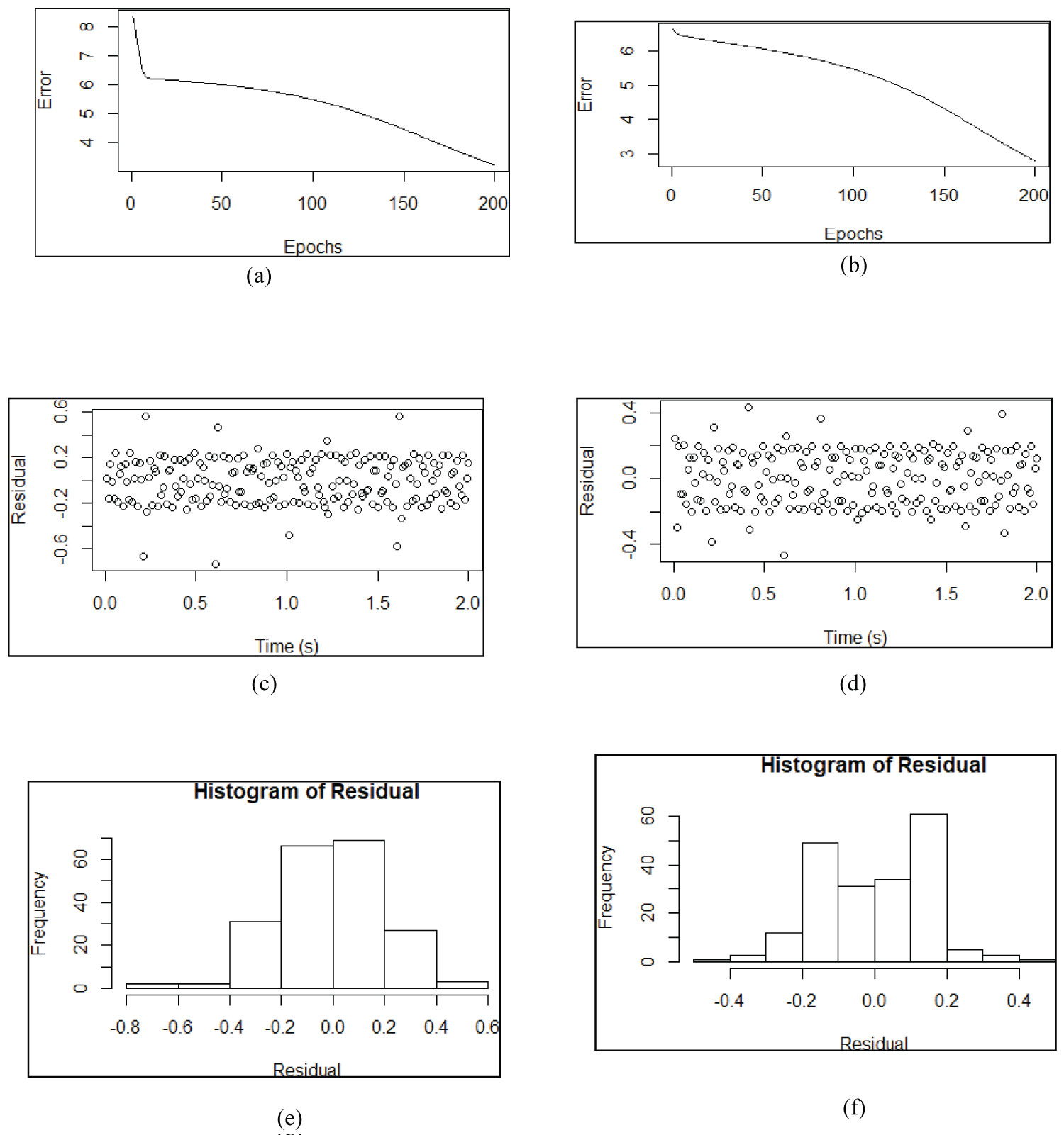
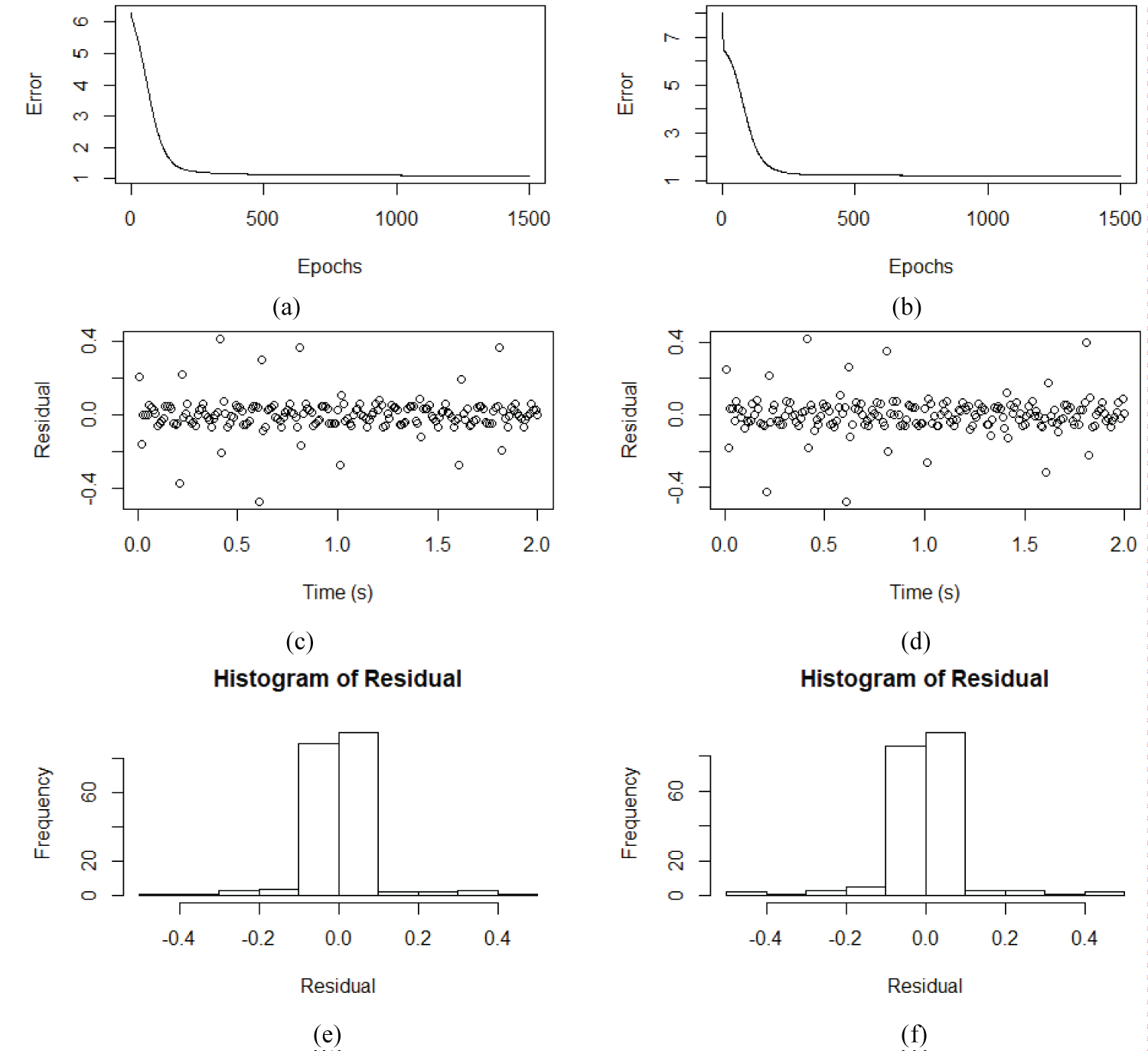
Figure 2a and Figure 2b show the early stopping for the RNN training with 10 hidden nodes. As can be seen the error decay has reached the value ≅ 3 and stabilized after 200 epochs, approximately. Figure 2a displays the standard deviation (σ) equal to zero in the input data $(a_0,a_1,and{b}_1)$ and Figure 2b shows the input data with σ = 0.001.

Figure 2c and Figure 2d show the early stopping for the RNN training. Figure 2c displays the residual i.e., the difference the expected values for the flap motion and the obtained values of the RNN. Figure 2d shows residual versus time (s) the input data with σ = 0.001. The histogram of the residual shown in Figure 2c is displayed in Figure 2e, the standard deviation of the histogram is 0.16. The corresponding histogram of the residual for Figure 2d is plotted in Figure 2e; in this case, the standard deviation of the histogram is 0.19.

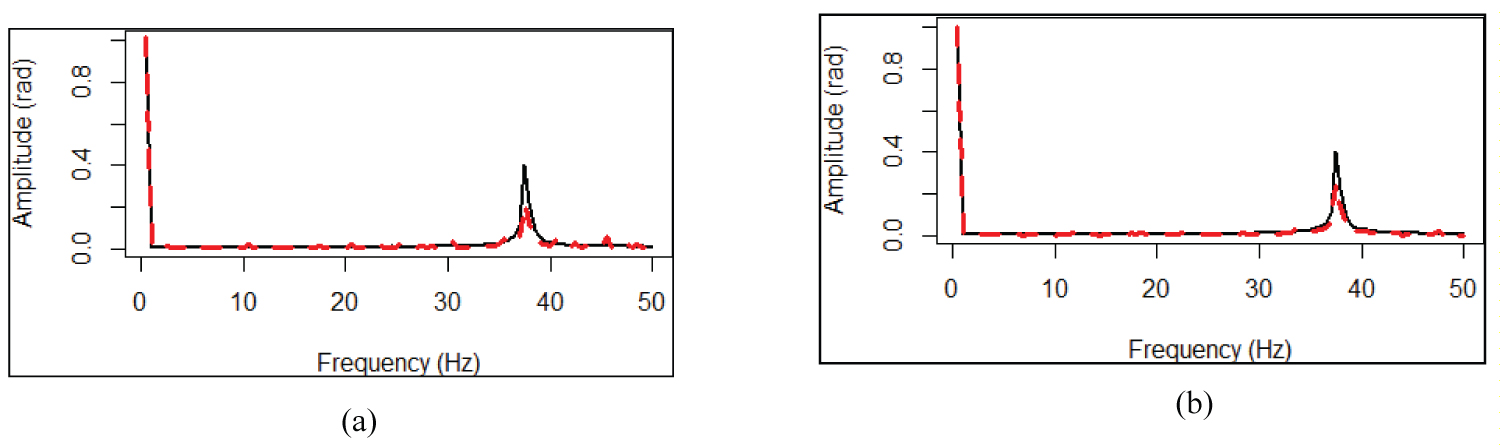
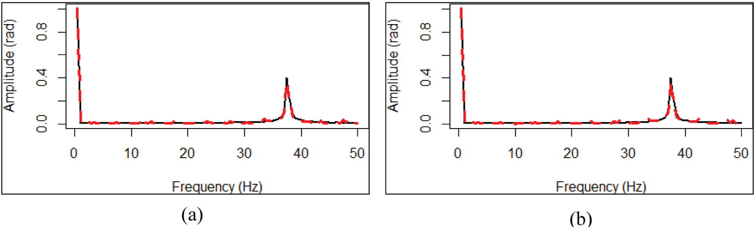
Furthermore, the signals have been analysed in the frequency domain. Figure 3a displays the frequency spectrum of the flap motion response (dotted black line) and the standard deviation (σ) is equal to zero in the input data. The normalized spectrum from simulated and emulated response by the RNN model asserts that the network model is capable of capturing the system frequency contents. It is shown that the frequency content in the simulated response is identified in the RNN plotted with a dotted red line, both signal display a main peak of frequency around 37.1 Hz, which is the tail rotor frequency. Figure 3b shows the frequency spectrum of the flap motion response (dotted black line) and the standard deviation (σ = 0.001) in the input data. The normalized spectrum from simulated and emulated response by the RNN model asserts that the network model is capable of capturing the system frequency contents. It is displayed that the frequency content in the simulated response is identified in the RNN plotted with a dotted red line, both signal display a main peak of frequency around 37.1 Hz, which is the tail rotor frequency.

Fitting

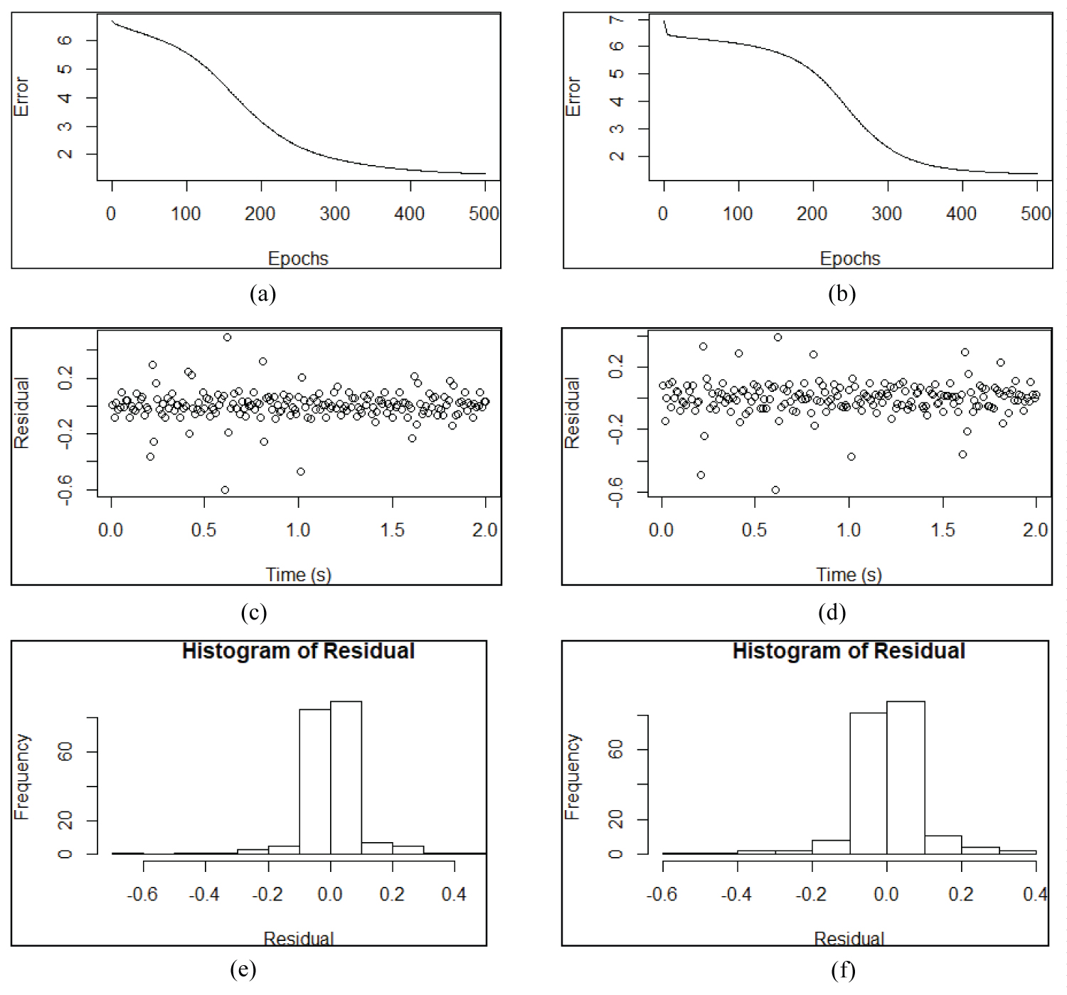
Figure 4a and Figure 4b show the fitting for the RNN training with 10 hidden nodes. As can be seen the error decay has reached the value ≅ 1 and stabilized after 500 epochs, approximately. Figure 4a displays the standard deviation (σ) equal to zero in the input data and Figure 4b shows the input data with σ = 0.001.

Figure 4c and Figure 4d show the fitting for the RNN training. Figure 4c displays the residual i.e., the difference the expected values for the flap motion and the obtained values of the RNN. Figure 4d shows residual versus time (s) the input data with σ = 0.001. The histogram of the residual shown in Figure 4c is displayed in Figure 4e, the standard deviation of the histogram is 0.10. The corresponding histogram of the residual for Figure 4d is plotted in Figure 4e, in this case, the standard deviation of the histogram is 0.10.

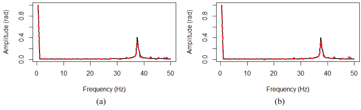
Furthermore, the signals have been analyzed in the frequency domain. Figure 5a displays the frequency spectrum of the flap motion response (dotted black line) and the standard deviation (σ) is equal to zero in the input data. The normalized spectrum from simulated and emulated response by the RNN model asserts that the network model is capable of capturing the system frequency contents. It is shown that the frequency content in the simulated response is identified in the RNN plotted with a dotted red line, both signal display a main peak of frequency around 37.1 Hz, which is the tail rotor frequency. Figure 5b shows the frequency spectrum of the flap motion response (dotted black line) and the standard deviation (σ = 0.001) in the input data. The normalized spectrum from simulated and emulated response by the RNN model asserts that the network model is capable of capturing the system frequency contents. It is displayed that the frequency content in the simulated response is identified in the RNN plotted with a dotted red line, both signal display a main peak of frequency around 37.1 Hz, which is the tail rotor frequency.

Overfitting

Figure 6a and Figure 6b show the fitting for the RNN training with and 20 hidden nodes. As can be seen the error decay has reached the value ≅ 1 and stabilized after 1500 epochs, approximately. Figure 6a displays the standard deviation (σ) equal to zero in the input data $\left(a_0,a_1,and{b}_1\right)$ and Figure 6b shows the input data with σ = 0.001.

Figure 6c and Figure 6d show the fitting for the RNN training. Figure 6c displays the residual i.e., the difference the expected values for the flap motion and the obtained values of the RNN. Figure 6d shows residual versus time (s) the input data with σ = 0. 001. The histogram of the residual shown in Figure 6c is displayed in Figure 6e, the standard deviation of the histogram is 0.09. The corresponding histogram of the residual for Figure 6d is plotted in Figure 6e, in this case, the standard deviation of the histogram is 0.09.

Furthermore, the signals have been analysed in the frequency domain. Figure 7a displays the frequency spectrum of the flap motion response (dotted black line) and the standard deviation (σ) is equal to zero in the input data. The normalized spectrum from simulated and emulated response by the RNN model asserts that the network model is capable of capturing the system frequency contents. It is shown that the frequency content in the simulated response is identified in the RNN plotted with a dotted red line, both signal display a main peak of frequency around 37.1 Hz, which is the tail rotor frequency. Figure 7b shows the frequency spectrum of the flap motion response (dotted black line) and the standard deviation (σ = 0.001) in the input data. The normalized spectrum from simulated and emulated response by the RNN model asserts that the network model is capable of capturing the system frequency contents. It is displayed that the frequency content in the simulated response is identified in the RNN plotted with a dotted red line, both signal display a main peak of frequency around 37.1 Hz, which is the tail rotor frequency.

As a consequence, the input data with σ = 0.001 have been used for training RNN. The possibility of using this approach in situations wherein specific previous information about the training data can be incorporated is suitable and can be used in further studies.

Conclusions

The main contribution of this work is to present the training outcomes of a RNN for a helicopter tail rotor. The main interest of this ANN is the capability of representing the flap motion, which often, is difficult to get under determined dynamics conditions. The model has been derived to focus the study on the system's own dynamics only.

In summary, the work here presented provides a method for the cumbersome task of representing a realistic and high-fidelity rotorcraft tail rotor model considering the dynamics. Being this software tool a suitable environment for engineers in this field. A study for the tail rotor flap motion was done by using a RNN in order to open the door to the helicopter design as well as to establish the basis of future works.

References

1. Ganguli R, Chopra I, Hass D J (1998) Helicopter rotor system fault detection using physics-based model and neural networks. AIAA Journal 36: 1078-1086.
2. Sadati N, Faghihi A H (2006) Neural networks in identification of helicopters using passive sensors. Systems, man and cybernetics, IEEE International Conference.
3. Zhang HB, Ju YQ, Cao XF, et al. (2014) Helicopter reliability researching based on neural networks. Applied Mechanics and Materials 651-653: 747-750.
4. Lee A, Habtour E, Gadsden SA (2016) Proposed health state awareness of helicopter blades using an artificial neural network strategy. Proc SPIE 9872.
5. Dellomo M R (1999) Helicopter gearbox fault detection: A neural network-based approach. J Vib Acoust 121: 265-272.
6. Hunt K J, Sbarbaro D, Zbikowski R, et al. (1992) Neural networks for control systems - a survey. Automatica 28: 1083-1112.
7. Vyas NS, Satishkumar D (2001) Artificial neural network design for fault identification in a rotor-bearing system. Mechanism and Machine Theory 36: 157-175.
8. Marques FD, Rodrigues de Souza LF, Rebolho DC, et al. (2005) Application of time-delay neural and recurrent neural networks for the identification of a hingeless helicopter blade flapping and torsion motions. J Braz Soc Mech Sci Eng 27: 97-103.
9. Johnson W (1980) Helicopter theory Princeton Univ Press Princeton NJ.
10. Watkinson J (2004) The art of the helicopter. Elsevier Butterworth-Heinemann.
11. Leishman JG (2007) Principles of helicopter aerodynamics. Cambridge University Press.
12. Newman S (1994) The Foundations of Helicopter Flight. Edward Arnold.
13. Bramwell ARS, Done G, Balmford D (2001) Bram well's helicopter dynamics. Butterworth-Heinemann.
14. Pad field GD (2007) Helicopter Flight Dynamics: The theory and application of flying qualities and simulation modelling. Blackwell Publishing.
15. Zhang L, Suganthan PN (2016) A survey of randomized algorithms for training neural networks. Information Sciences 364-365: 146-155.