On a Method of Lagrange Multipliers for Cruise Drag Minimization

Abstract

A blended-wing-body is an example of an aircraft configuration with multiple control surfaces. The most effective use of these control surfaces, e.g. to minimize cruise drag due to pitch trim, or to maximize pitching moment at low speed in an engine-out condition, leads to optimization problems. This kind of control optimization problems can be addressed by the method of Lagrange multipliers; this allows for multiple constraints, e.g. constant lift, pitching or other moments, each associated with one multiplier. The value of the multiplier is a measure of the severity of the constraint, e.g. the drag penalty of imposing pitch trim at constant lift. The estimates of the Lagrange multipliers for different control surfaces also indicate the evolution of the iterative process to find the optimum. Three distinct initial conditions to start the iterative process are considered. The method is applied to multiple control surfaces, taking into account their mutual interactions and also the influence of shifts of center of gravity. It is shown in particular cases that it is possible to achieve pitch trim in cruise with drag reduction relative to the untrimmed case.

Keywords

Multiple control surfaces, Flying-wing configuration, Optimization, Cruise drag, Pitch trim, Lagrange multiplier

Nomenclature

List of symbols indicating the first equation where each symbol is defined of first appears:

$\overline{c}$ : Mean Aerodynamic Chord: (2a)

$C_D$ : Drag Coefficient: (25)

$C_{D_i}$ : Drag Coefficient of the Control Surface i: (2b)

${C^{\prime }}_{D_i}$ : First-order derivative of the drag coefficient with regard to the deflection of the control surface i: (3a, 9a)

${C^{\prime }}_{D_{ij}}$ : First-order derivative of the drag coefficient of the control surface i with regard to the deflection of control surface j: (15a)

${C^{″}}_{D_i}$ : Second-order derivative of the drag coefficient with regard to the deflection of control surface i: (12a)

$C_L$ : Lift Coefficient: (6b)

$C_{L_i}$ : Lift Coefficient of Control Surface i: (19)

${C^{\prime }}_{L_i}$ : First-order derivative of the lift coefficient with regard to the deflection of control surface i: (20b)

$C_M$ : Pitching Moment Coefficient: (26c)

$C_{M_i}$ : Pitching moment coefficient of the control surface i: (2a)

${C^{\prime }}_{M_i}$ : First-order derivative pitching moment coefficient with regard to the deflection of the control surface i: (3b, 9b)

${C^{\prime }}_{M_{ij}}$ : First-order derivative of pitching moment coefficient of the control surface i with regard to the deflection of control surface j: (15b)

${C^{″}}_{M_i}$ : Second-order derivative of the pitching moment coefficient with regard to the deflection of control surface i: (12b; 66b)

${C^{″}}_{M_{ijk}}$ : Second-order derivative of the pitching moment coefficient of control surface i with regard to the deflections of control surfaces j and k: (66b)

$D$ : Trim Drag: (2b)

$D^{*}$ : Trim drag per unit dynamic pressure: (2b)

$D_{\min }^{*}$ : Minimum Trim Drag: (9)

${\overline{l}}_i$ : Moment arm of the control surface i relative to the reference c.g. position: (21a)

$l_i$ : Moment arm of the control surface i after shift of c.g. position: (21a)

$L$ : Lift: (19)

$L^{*}$ : Lift per unit dynamic pressure: (19)

$M$ : Pitching Moment: (2a)

$M^{*}$ : Pitching moment per unit dynamic pressure and mean aerodynamic chord: (2a)

$M_{\max }^{*}$ : Maximum pitching moment: (4)

I_ab : Identity Matrix: (17a)

q : Dynamic Pressure: (1)

U : Airspeed: (1)

$S_i$ : Area of the control surface i: (2a)

$S_0$ : Total Control Surface Area: (26d)

S: Wing Area: (25)

α : Angle of Attack: (26a)

α₀ : Cruise Angle of Attack: (26a)

${\delta }_i$ : Deflection of the control surface i: (2a)

${\overline{\delta }}_i$ : Optimal deflection of the control surface i: (5b)

$\lambda$ : Lagrange multiplier: (5a)

$\rho$ : Mass density of atmospheric air: (1)

$\Delta x_{cg}$ : Deviation from c.g. position l_i of the control surface i: (21a)

Abbreviations

AOA: Angle of Attack

BWB: Blended Wing Body

c.g.: Center of Gravity

FW: Flying-Wing

Ma: Mach Number

Introduction

Minimizing drag in cruise is most important for aircraft emissions and economics since this is the longest phase of most flights, and where a large proportion of the total fuel is burnt. It is therefore desirable to achieve pitch trim at cruise with the smallest possible drag penalty relative to the untrimmed aircraft; even better would be to achieve pitch trim in cruise with a drag reduction relative to the untrimmed aircraft. Thus, the subject of cruise drag minimization has received considerable attention in the literature, using a variety of methods [1-5]. There is a limited choice of control surfaces in the traditional aircraft configuration, with a fuselage to carry payload, a wing to carry fuel and wing to provide lift and roll control, and an empennage to provide yaw and pitch control. In a blended wing body (BWB) configuration, with control surfaces both on the centerbody and wing, there are multiple control surfaces; thus arises the question of which is the best combination of all available control surfaces to achieve pitch trim with least drag. The BWB offers superior lift-to-drag ratio over conventional configurations, promising lower fuel consumption; these benefits will be achieved more fully by minimization of any additional drag due to pitch trim in cruise [6-9]. This is an instance of flight control and stability with multiple controls [10-17] that is particularly relevant to novel aircraft designs like flying wing [18-39] and box-wing [40,41] aircraft. It falls into the broader scope of optimization and variational methods [42-54].

The method to be presented applies to the trimming of an aircraft, for any axis and any flight phase, when there is a choice of control surfaces to be used. It allows distinct control surfaces to have different deflections, in order to minimize drag, for a given constant control moment e.g. in cruise. Conversely, e.g. in a low-speed engine-out condition, with a given drag, it specifies the maximum control moment available [55]. It is shown that these two reciprocal problems have the same solution using Lagrange multipliers (section 2). An iterative procedure to find the optimal control surface deflection is presented (section 3). It is generalized (section 4) to coupled control surfaces and to the case where additional quantities should be conserved, e.g. lift. The optimization procedure is iterative and needs an initial condition to start. In order to have the starting values for the optimization procedure, the cruise condition of a flying-wing (FW) or Blended Wing Body (BWB) configuration is trimmed using the elevator alone (strategy A); the optimization method (strategy B) moves away from this initial condition and uses deflections of all five sets of control surfaces (section 5). The methods I and II achieve pitch trim without conserving lift and thus imply a change of flight condition, e.g. altitude or speed change or a combination of the two. To make a meaningful comparison between optimal and non-optimal methods of pitch trim in cruise with minimum drag, the methods I and II are modified into respectively strategies C and D both preserving lift, and thus not changing the cruise altitude or speed (section 6). The conclusion (section 7) compares the results of optimal and non-optimal strategies, with further details of the optimization methods in the appendix.

The main distinguishing features of the method of Lagrange multipliers compared with other optimization methods result from two properties of the multipliers. First, the magnitude of each multiplier indicates the importance of the constraint it is associated with: (i) A small Lagrange multiplier means that changing the constraint has little effect on the result of the optimization; (ii) On the contrary, a large Lagrange multiplier means that relaxing the constraint will lead to a significantly better result, and tightening the constraint will significantly degrade the result. In the case of partial Lagrange multipliers for each control surface, the optimum is when they are all equal, implying that: (i) If there are large differences the control surface deflections should be changed in a way that reduces those differences; (ii) As the differences between partial multipliers reduce the optimum comes closer. The computational cost of the algorithm is small (seconds in a PC) and the iterations map a neighborhood of the optimum.

2. Two Reciprocal Optimization Problems

Two reciprocal optimization problems in flight dynamics are: (i) For a given pitching moment, find the control surface deflections which minimize drag; (ii) For a given drag, find the control surface deflections which give maximum pitching moment. These two reciprocal problems correspond to: (i) the minimum drag due to pitch trim in cruise (subsection 2.1) and (ii) the maximum pitching moment in an engine-out low-speed condition (subsection 2.2). They have a similar solution (subsection 2.3) in terms of Lagrange multipliers but differ in the additional constraint.

2.1 Minimum cruise drag due to pitch trim

Denoting by q the dynamic pressure:

$$q\equiv \frac{1}{2}\rho U^2\text{ (1)}$$

the pitching moment per unit dynamic pressure and mean aerodynamic chord $\overline{c}$ is given by:

$$M*\equiv M/q\overline{c}={\displaystyle \sum _{i=1}^N{S}_i{C}_{M_i}\left({\delta }_i\right)}\text{ (2a)}$$

where: (i) The sum extends to all N control surfaces, $i=1,\mathrm{...},N$, e.g. $i=1$ is the elevator, and $i=2,\mathrm{...},N$ other surfaces which can be used for pitch control; (ii), $S_i$ is the area, $C_{M_i}$ the pitch control coefficient and ${\delta }_i$ is the deflection of the surface $i$. The trim drag per unit dynamic pressure is:

$$D*\equiv D/q={\displaystyle \sum _{i=1}^N{S}_i{C}_{D_i}\left({\delta }_i\right)}\text{ (2b)}$$

where $C_{D_i}$ is the dimensionless drag coefficient. The aim is to choose ${\delta }_i$ with $i=1,\mathrm{...},N$, so that, for a given pitching moment (2a), the drag (2b) is minimum.

2.2 Maximum pitching moment in engine-out condition

The condition of minimum drag (2b) requires that $D*$ be stationary

$$\text{d}D*=0:{\displaystyle \sum _{i=1}^N{S}_i{C^{\prime }}_{D_i}\text{d}{\delta }_i}=0\text{ (3a)}$$

where ${C^{\prime }}_{D_i}\equiv \text{d}{C}_{D_i}/\text{d}{\delta }_i$ and it is assumed that $C_{D_i}$ depends only on the deflection of the corresponding surface ${\delta }_i$ (this will be generalized to coupled control surfaces in subsection 4.1). However, the deflections ${\delta }_i$ are not independent, because they must keep the pitching moment (2a) constant:

$M*=const.:{\displaystyle \sum _{i=1}^N{S}_i{C^{\prime }}_{M_i}\text{d}{\delta }_i}=0\text{ (3b)}$

The reciprocal problem, e.g. corresponding to an engine-out condition, is for a given drag $D*$ to maximize the pitching moment:

$\left(D_{\min }^{*},M^{*}=const\right)\iff \left(D^{*}=const,M_{\max }^{*}\right)\text{ (4)}$

and it leads to the set of same equations (3a,b). Thus, apart from a distinct constraint, both problems have a similar solution, i.e. lead to a set of optimal control surface deflections, which are determined next by the method of Lagrange multipliers.

2.3 Optimal control surface deflection and Lagrange multiplier

Introducing the Lagrange multiplier $\lambda$, the equation (3a) is multiplied by $\lambda$ and (3b) is added:

$${\displaystyle \sum _{i=1}^N{S}_i\left({C^{\prime }}_{D_i}\lambda +{C^{\prime }}_{M_i}\right)\text{d}{\delta }_i}=0\text{ (5a)}$$

Now there are $N+1$ unknowns: (i) the $N$ deflections ${\delta }_i$ of the control surfaces; (ii) the multiplier $\lambda$. If the deflections are taken as independent in (5a) then follow $N$ optimization equations:

$$-\lambda {C^{\prime }}_{D_i}\left({\overline{\delta }}_i\right)={C^{\prime }}_{M_i}\left({\overline{\delta }}_i\right)\text{ (5b)}$$

where the ${\delta }_i$ appears implicitly in the derivatives of the drag ${C^{\prime }}_{D_i}$ and moment ${C^{\prime }}_{M_i}$ coefficients; the subsidiary condition is the conservation of the pitching moment (3b), and it is the $\left(N+1\right)-th$ equation. From the N+1 equations (5b) + (3b), can be determined the $N$ optimal deflections ${\overline{\delta }}_i$ and the optimal Lagrange multiplier $\overline{\lambda }$. Once these are known, the minimum trim drag follows from:

$$D_{\min }^{*}={\displaystyle \sum _{i=1}^N{S}_i{C}_{D_i}\left({\overline{\delta }}_i\right)}\text{ (6)}$$

using the optimal deflections ${\overline{\delta }}_i$. The optimal Lagrange multiplier $\overline{\lambda }$ indicates how much the constraint of constant pitching moment $M^{*}$ penalizes the minimum drag $D^{*}$, i.e. a large $\overline{\lambda }$ indicates a large effect on drag $D_{*}^{}$ to achieve the required pitching moment $M^{*}$ and a small $\overline{\lambda }$ indicates a small effect on drag.

3. The Method of Solution for the Optimal Deflections

The direct (or minimum drag) and reciprocal (or maximum pitching) moment problems, lead to distinct optimal deflections (subsection 3.1) because the subsidiary condition is different. The optimization conditions are the same (subsection 3.2) and lend themselves to a similar iterative method of solution (subsection 3.3).

3.1 Direct and reciprocal optimization problems

In the case of the reciprocal problem the same N+1 unknowns, the N optimal control surface deflections ${\overline{\overline{\delta }}}_i$ and Lagrange multiplier $\overline{\overline{\lambda }}$ are determined from N+1 conditions: (i) The same N optimization conditions (5b); (ii) The different condition (3a) of constant drag instead of constant pitching moment (3b). The maximum pitching moment is given (2a) by:

$$M_{\max }^{*}={\displaystyle \sum _{i=1}^N{S}_i{C}_{M_i}\left({\overline{\overline{\delta }}}_i\right)}\text{ (7)}$$

Thus the direct (subsection 2.1) [ inverse subsection 2.2)] problems use the same N optimization conditions (5b), and a distinct subsidiary condition of constant pitching moment (3b) [constant drag (3a)] and thus lead to a different set of optimal deflections ${\overline{\delta }}_i\left({\overline{\overline{\delta }}}_i\right)$ and a distinct Lagrange multiplier $\overline{\lambda }\left(\overline{\overline{\lambda }}\right)$:

$$\left\{\left(5b\right)+\left(3b\right),{\overline{\delta }}_i,\overline{\lambda }\right\}\iff \left\{\left(5b\right)+\left(3a\right),{\overline{\overline{\delta }}}_i,\overline{\overline{\lambda }}\right\}\text{ (8)}$$

In what follows the direct problem will be considered explicitly; similar reasonings would apply to the reciprocal problem. Note that the optimization conditions (5b) involve the first derivative of the drag $C_{D_i}$ and pitching moment $C_{M_i}$ coefficients with regard to the deflections:

$${C^{\prime }}_{D_i}\equiv \text{d}{C}_{D_i}/\text{d}{\delta }_i,{C^{\prime }}_{M_i}\equiv \text{d}{C}_{M_i}/\text{d}{\delta }_i\text{ (9a,b)}$$

where it is assumed that the control surfaces are independent, i.e. each $C_{D_i}$, $C_{M_i}$ depends only in the corresponding ${\delta }_i$, and it is not affected by other ${\delta }_j$ with $i\ne j$. This restriction will be lifted in subsection 4.1.

3.2 Iterative method of solution

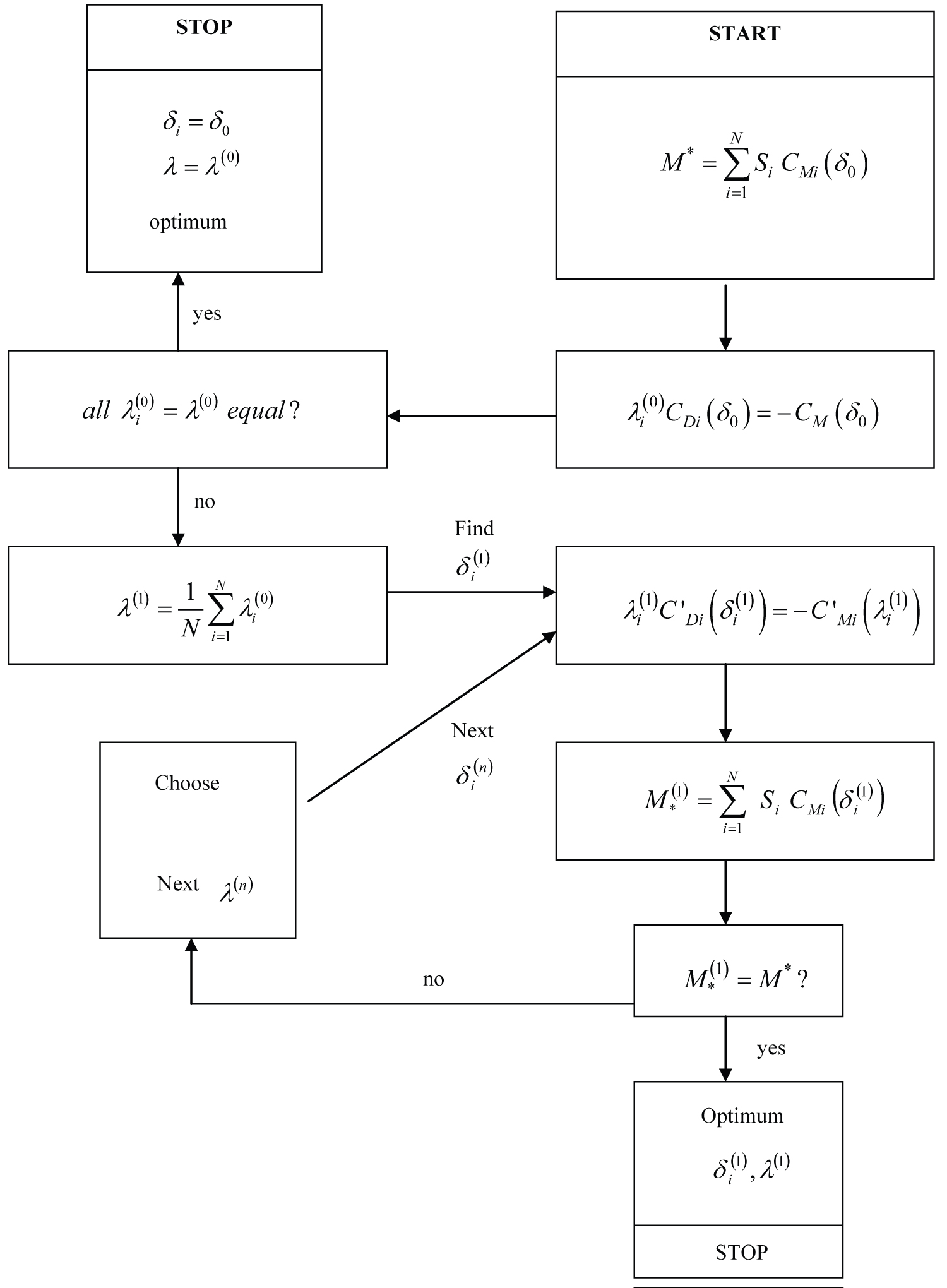
The key to the solution of the direct and inverse optimization problems is to find the optimal deflections ${\overline{\delta }}_i$ and multiplier $\overline{\lambda }$ which satisfy the N optimization equations (5b) plus the subsidiary condition of constant pitching moment (3a). This is an implicit system, which can be solved iteratively (Figure 1) as follows: (i) Start with equal deflections for all surfaces ${\delta }_i^{\left(0\right)}={\delta }_0$, for the given pitching moment (2a):

${\delta }_i^{\left(0\right)}={\delta }_0:M*={\displaystyle \sum _{i=1}^N{S}_i{C}_{M_i}\left({\delta }_0\right)}\text{ (10a)}$

(ii) The N+1 control equations (5b) specify N+1 first estimates of the multiplier:

$${\lambda }_i^{\left(0\right)}=-{C^{\prime }}_{M_i}\left({\delta }_0\right)/{C^{\prime }}_{D_i}\left({\delta }_0\right)\text{ (10b)}$$

(iii) If all ${\lambda }_i^{\left(0\right)}\equiv {\lambda }_{}^{\left(0\right)}$ are equal, we have the optimal solution ${\delta }_{0i}={\delta }_0$, $\lambda ={\lambda }^{\left(0\right)}$, which satisfies all N+1 equations (3a,5b), implying that the minimum drag would occur for equal deflections of all control surfaces; (iv) Most likely this is not the case, so if the ${\lambda }_i^{\left(0\right)}$ are not all equal, their arithmetic mean is taken as the next iteration:

$${\lambda }^{\left(1\right)}=\frac{1}{N}{\displaystyle \sum _{i=1}^N{\lambda }_i^{\left(0\right)}}\text{ (11)}$$

(v) Substituting ${\lambda }^{\left(1\right)}$ in the N optimization equations (5b), gives the next iteration for the deflections ${\delta }_i^{\left(1\right)}$, which are generally distinct; (vi) Substituting the ${\delta }_i^{\left(1\right)}$ in the pitching moment (2a) leads to a value $M^{\left(1\right)}$, which is the optimum if $M^{\left(1\right)}=M_{*}$ has the required value $M_{*}$; (vii) If not ${\lambda }^{\left(1\right)}$ is modified to ${\lambda }^{\left(2\right)}$ and the process continued until $M^{\left(n\right)}\to M_{*}$. The modification process for the Lagrange multiplier at the iteration n+1 could be as in (11) the arithmetic mean of the preceding $n^{\text{th}}$ iteration. The iterative algorithm initiated with equation (10a) followed by equations (10b) and (11) consists of simple algebraic operations and a few choices indicated in the Figure 1. A cycle can be performed in a PC in less than a second, and thus computational cost is not a issue, even for a large number of iterations, that should not be necessary in most cases. A larger number of iterations will require more care with numerical bounding-off errors.

3.3 Linear and non-linear optimization equations

The critical step in iterative method of solution is to solve the optimization equation (5b) for the deflections ${\delta }_i$. This is analysed next. If the drag $C_{D_i}$ and control $C_{M_i}$ coefficients are linear in the deflections ${\delta }_i$, then (9a,b) are constants, and generally there is not a single value $\lambda$ of the Lagrange multiplier which will satisfy all N relations (5b). Thus, there is no optimum. It follows that optimal deflections exist only if the drag or control coefficients are non-linear functions of the control surface deflections, e.g.:

$$C_{D_i}\left({\delta }_i\right)=C_{D_{0i}}+{C^{\prime }}_{D_{0i}}{\delta }_i+\frac{1}{2}{\left({\delta }_i\right)}^2{C^{″}}_{D_{0i}}\text{ (12a)}$$

$$C_{M_i}\left({\delta }_i\right)=C_{M_{0i}}+{C^{\prime }}_{M_{0i}}{\delta }_i+\frac{1}{2}{\left({\delta }_i\right)}^2{C^{″}}_{M_{0i}}\text{ (12b)}$$

in a quadratic case. In this case the optimization conditions are specified substituting (12a,b) in (5b):

$$-\lambda \text{}\left({C^{\prime }}_{D_{0i}}+{\delta }_i{C^{″}}_{D_{0i}}\right)={C^{\prime }}_{M_{0i}}+{\delta }_i{C^{″}}_{M_{0i}},\text{ (13a)}$$

and can be solved for the deflections:

$-{\delta }_i=\frac{{C^{\prime }}_{M_{0i}}+\lambda {C^{\prime }}_{D_{0i}}}{{C^{″}}_{M_{0i}}+\lambda {C^{″}}_{D_{0i}}}\text{ (13b)}$

thus the optimum exists, as specified by (13b).

4. Extension to Coupled Surfaces and Additional Constraints

The preceding method is extended in two ways: (i) To coupled control surfaces (subsection 4.1), such that the drag $C_{D_i}$ and pitching moment $C_{M_i}$ coefficients of surface i depend on the defections ${\delta }_j$ of other surfaces; (ii) To additional constraints (subsection 4.2), e.g., a condition of constant lift. The two generalizations can be taken together, and it is important to note that the optimization problem depends on the position of c.g., allowing an approximation for (subsection 4.3) small deviation.

4.1 Optimization condition for the coupled control surfaces

In the case of coupled control surfaces the drag coefficient $C_{D_i}$ of surface i depends on the defections ${\delta }_j$ of all control surfaces:

$$D^{*}={\displaystyle \sum _{i=1}^N{C}_{D_i}\left({\delta }_j\right)}{S}_i\text{ (14a)}$$

and the condition of minimum (or constant) drag:

$$0=\text{d}{D}^{*}={\displaystyle \sum _{i,j=1}^N{C^{\prime }}_{D_{ij}}}{S}_i\text{d}{\delta }_j\text{ (14b)}$$

involves matrices of first-order derivatives (15a):

${C^{\prime }}_{D_{ij}}\equiv \partial C_{D_i}/\partial {\delta }_j,{C^{\prime }}_{M_{ij}}\equiv \partial C_{M_i}/\partial {\delta }_j\text{ (15a,b)}$

and likewise for the pitching moment (15b). If follows that the optimization conditions (5b) are now:

$$0=\text{d}{M}^{*}+\lambda \text{d}{D}^{*}={\displaystyle \sum _{i=0}^N{S}_i{\displaystyle \sum _{j=1}^N\left({C^{\prime }}_{M_{ij}}+\lambda {C^{\prime }}_{D_{ij}}\right)}\text{d}{\delta }_j};\text{ (16a)}$$

since the variations of the deflections cannot be all zero, the determinant must vanish:

$$\left(\text{d}{\delta }_1,\text{d}{\delta }_2,\mathrm{...},\text{d}{\delta }_N\right)\ne \left(0,0,\mathrm{...},0\right):\text{ det}\left({C^{\prime }}_{M_{ij}}+\lambda {C^{\prime }}_{D_{ij}}\right)=0.\text{ (16b)}$$

Thus minus the Lagrange multiplier λ is minus an eigenvalue of the pair of matrices ${C^{\prime }}_{M_{ij}}$ and ${C^{\prime }}_{D_{ij}}$. If the eigenvalues are distinct then the eigenvectors are orthogonal. In this orthogonal frame, with indices a, b, the matrices became diagonal:

$$C{\text{'}}_{D_{ab}}=C{\text{'}}_{D_a}{I}_{ab},C{\text{'}}_{M_{ab}}=C{\text{'}}_{M_a}{I}_{ab},\text{ (17ab)}$$

where I_ab is the identity matrix; thus (16a) show that:

$$0=d{M}^{*}+\lambda d{D}^{*}={\displaystyle \sum _{a=1}^N{S}_{a}d{\delta }_a\left({C^{\prime }}_{M_a}+\lambda {C^{\prime }}_{D_a}\right)};\text{ (18)}$$

the controls are now decoupled as in (5b). Hence the analysis of (subsection 3.3) applies again, to show that an optimum exists for non-linear controls, e.g. (13b) in the quadratic case (12a,b).

4.2 Flight at varying speed/altitude or constant lift

The lift per unit dynamic pressure induced by the control surfaces is given by:

$$L^{*}=L/q={\displaystyle \sum _{i=1}^N{C}_{L_i}{S}_i}\text{ (19)}$$

where $C_{L_i}$ is the lift coefficient of control surface i. In the preceding optimization problem, the optimal deflections ${\overline{\delta }}_i$ would generally lead to a change in lift to $L^{*}$, implying flight at a different dynamic pressure (1), i.e. either speed or altitude or both will change, viz.: (i) If lift was increased ${\overline{L}}^{*}>L^{*}$, then the aircraft would descend to a lower altitude, corresponding to a larger atmospheric mass density $\rho$, or fly faster, leading to a combination such that lift equals weight again; (ii) If lift was decreased, then the aircraft would fly at higher altitude, or slower.

If it is required to keep flight altitude and speed, then the constraint of constant lift can be introduced via an additional Lagrange multiplier µ relative to (16a), viz.:

$$0=\text{d}{M}^{*}+\lambda \text{d}{D}^{*}+\mu \text{d}{L}^{*}\text{ (20a)}$$

and the optimization condition (5b) would be replaced by:

$0={C^{\prime }}_{M_i}+\lambda {C^{\prime }}_{D_i}+\mu {C^{\prime }}_{L_i}\text{ (20b)}$

for decoupled control surfaces (subsection 3.3). In the case of coupled control surfaces (subsection 4.1) the relations (20b) would hold after diagonalization, similar to (17a,b) also for ${C^{\prime }}_{L_{ab}}$. The iterative method of solution (subsection 3.2) would again apply, with two multipliers $\lambda ,\mu$. Any additional constraint would add another multiplier.

The drag minimization with constant pitch trim and multiple control surfaces (section 2) has been extended to: (i) take into account the coupling between control surfaces (subsection 4.1); (ii) the additional constraint of constant lift (subsection 4.2) to ensure unchanged cruise speed or altitude. Next (subsection 4.3) is considered not a further variation of the optimization problem, but rather the consequences of c.g. changes on the optimal deflections.

4.3 Effect on the optimization of large and small c.g. shifts

The preceding calculations involve the c.g. position in two ways: (i) The moment arm ${\overline{l}}_i$ can be calculated for $l_i$ a given c.g. position (e.g. 25% of mean aerodynamic chord) and then corrected for the c.g. deviation $\Delta x_{cg}$ from this position (27a):

$${\overline{l}}_i=l_i-\Delta x_{cg};{\left(\Delta x_{cg}\right)}^2<<{\left(l_i\right)}^2;\text{ (21a,b)}$$

(ii) If the c.g. position shift is small (21b) relative to the moment arm, then the aerodynamic coefficients are not affected. The pitching moment (2a) is now taken for unit dynamic pressure:

$$M^{**}/q={\displaystyle \sum _{i=1}^N{l}_i{S}_i{\overline{C}}_{Mi}\left({\delta }_i\right)}\text{ (22)}$$

and the moment arms $l_i$ introduced instead of the mean aerodynamic chord $\overline{c}$; note that this changes the value of the pitching moment coefficient to ${\overline{C}}_{Mi}$. Using (13b) with $C_{M0i}$ replaced by $l_i{\overline{C}}_{M0i}$ leads to:

$$-{\delta }_i=\frac{{\overline{l}}_i\overline{C}{\text{'}}_{M_{0i}}+\lambda {C^{\prime }}_{D_{0i}}-x_{cg}\overline{C}{\text{'}}_{M_{0i}}}{{\overline{l}}_i\overline{C}{"}_{M_{0i}}+\lambda \overline{C}{"}_{D_{0i}}-x_{cg}\overline{C}{"}_{M_{0i}}}\text{ (23)}$$

where the aerodynamic coefficient may depend on the c.g. position. For small c.g. deviations (21b), the optimal deflections (23) linearize:

$$-{\delta }_i=\frac{{\overline{l}}_i\overline{C}{\text{'}}_{M_{0i}}+\lambda {C^{\prime }}_{D_{0i}}}{{\overline{l}}_i\overline{C}{"}_{M_{0i}}+\lambda {C^{″}}_{D_{0i}}}\left\{\begin{array}{l}1+x_{cg}\left[\frac{\overline{C}{"}_{M_{0i}}}{l_i\overline{C}{"}_{M_{0i}}+\lambda {C^{″}}_{D_{0i}}}-\frac{\overline{C}{\text{'}}_{M_{0i}}}{l_i\overline{C}{"}_{M_{0i}}+\lambda {C^{\prime }}_{D_{0i}}}\right]\\ +O\left({\left(x_{cg}\right)}^2\right)\end{array}\right\}(24)$$

where the aerodynamic coefficients are calculated for the reference c.g. position $x_{cg}=0$.

5. Initial Condition and Iterative Solution

Starting from a given cruise condition (subsection 5.1) pitch trim may be achieved by the strategy A (subsection 5.2) of deflection of the elevator alone, that is the most effective pitch control surface and simplest. This is used as the initial condition in the iterative application of the strategy B of Lagrange multipliers (Figure 1) towards optimal deflections (subsection 5.3).

5.1 Lift and drag in the cruise condition

Consider a BWB aircraft configuration at a cruise weight $W=715t$ intermediate between initial and final cruise weights. At cruise altitude z = 35 kft the sound speed is c = 295 m s^-1, and the cruise Mach number $Ma=0.85$ corresponds to a indicated airspeed $U=Ma\times c=251m{s}^{-1}$. At the tropopause, the mass density is ρ = 0.223 kg m^-3, and thus the dynamic pressure is $q=\frac{1}{2}\rho U^2=7.025\times {10}^{3}N{m}^{-2}$. For a reference wing area S = 961.35 m², this corresponds to a cruise lift coefficient:

$$C_L=2W/\left(\rho S{U}^2\right)=W/\left(qS\right)=\mathrm{0.10588.}\text{ (25)}$$

The lift coefficient C_L, and also the drag C_D and pitching moment C_M coefficients, are given in Table 1 for the chosen BWB aircraft configuration in a typical cruise condition. Linear interpolation of the values of the lift coefficient between zero α = 0° and three degree α = 3° AOA, shows from Table 1 that (25) corresponds to a cruise AOA

α₀ = 0.71789°,        (26a)

Further linear interpolation shows that this AOA corresponds to a cruise drag coefficient (26b)

C_D = 0.00569, CM = - 0.02441,        (26b,c)

and pitching moment coefficient (26c). The total dynamic force $\overline{q}=qS=6.7535\times {10}^{6}N,$ then leads to a cruise drag $D=C_D\overline{q}=3.8427\times {10}^{4}N$ and pitching moment $M=C_M\overline{q}\overline{c}=-5.2699\times {10}^6$ N m. The cruise lift-to-drag ratio is L/D = C_L/C_D = 18.6.

There are five sets i = 1,...,5 control surfaces available for pitch control whose areas are indicated in Table 2 together with the fraction of wing area Si/S, and fraction of total control surface are Si/S0, where:

$$S_0\equiv {\displaystyle \sum _{i=1}^5{S}_i}.\text{ (26d)}$$

The lift C_Li, drag C_Di and pitching moment C_Mi coefficients for each surface i = 1,...,5, and those for all surfaces together i = 0, are given in Table 3 for upward or downward deflections of three degrees δ_i = ± 3°, at angles of attack α = 0° and α = 3°. From these are interpolated the values at cruise AOA in (26a). The Table 4 repeats the values of the lift C_Li, drag C_Di and pitching moment C_Mi coefficients for all six cases i = 0,1,...,5 in cruise condition, for zero deflection δ_i = 0° and three degree deflection upward or downward δ_i = ± 3°, to calculate: (i) Two first-order central differences $\nabla C_{Xi}$ at deflections δ_i = ± 1.5°; (ii) One second-order central difference ∇² C_Xi at zero deflection δ_i = 0. The calculation is similar for lift X ≡ L, drag X ≡ D and pitching moment X ≡ M, and can be used to specify in Table 5: (i) Two values of the first-order derivative:

$$\begin{array}{l}{C^{\prime }}_{Xi}\left({\delta }_i=\pm 1.5º\right)=\pm \left[C_{Xi}\left({\delta }_i=\pm 3º\right)-C_{Xi}\left({\delta }_i=0º\right)\right]/3º\text{ (27a,b)}\\ \equiv \pm \nabla C_{Xi}\left(\delta =\pm {1.5}^o\right)/3º;\end{array}$$

(ii) One value of the second-order derivative:

$${C^{″}}_{Xi}\left({\delta }_i=0º\right)=\left[C_{Xi}^{"}\left({\delta }_i=1.5º\right)-C_{Xi}^{\text{'}}\left({\delta }_i=-1.5º\right)\right]/3º\equiv {\nabla }^2{C}_{Xi}\left(\delta =0º\right)/3º.\text{ (27c)}$$

The value of the second-order derivative is always taken to be (27c) in Table 5, because only one estimate is available. The first derivative can be interpolated between the two values (27a,b), or its mean value taken at zero deflection,

$$\begin{array}{l}{C^{\prime }}_{Xi}\left({\delta }_i=0º\right)=\left[{C^{\prime }}_{Xi}\left({\delta }_i=1.5º\right)+{C^{\prime }}_{Xi}\left({\delta }_i=-1.5º\right)\right]/2\text{ (28)}\\ =\left[C_{Xi}\left({\delta }_i=3º\right)-C_{Xi}\left({\delta }_i=-3º\right)\right]/6º,\end{array}$$

and is also indicated in Table 5. The preceding tables contain all the data needed to implement various trimming strategies for which different strategies are possible. The simplest (strategy A) is pitch trim by deflection of the elevator alone, that is the most effective control surface (subsection 5.2), and also serves as the initial condition for the strategy B of optimization (subsection 5.3).

5.2 Pitch trim using the elevator only

It is seen from Table 5, that the centerbody elevator has: (i) One of the largest positive pitching moment slopes, hence can trim the aircraft with smaller deflections; (ii) Has the largest (in modulus) negative drag slope, so that drag is reduced for small deflections. This suggests the strategy A of maximal deflection of the inboard control surfaces. The innermost trailing-edge control surface is the central body elevator, which would produce the required [(26c) or Table 1] pitching moment coefficient

$$\begin{array}{l}-C_M=C_{MR}\equiv 0.02441=C_{M1}\left({\delta }_I\right)\Rightarrow {\delta }_I=8.9798º\equiv {\delta }_{I1},(29a-c)\\ 0={\delta }_{I2}={\delta }_{I3}={\delta }_{I4}={\delta }_{I5},\end{array}$$

for a deflection (29b) which is calculated by linear interpolation from Table 4 as follows:

$${\delta }_{Ii}=\frac{0.02441-\left(-0.02441\right)}{0.00810-\left(-0.02441\right)}\times 3º=8.9798º\text{ (29d)}$$

the other control surfaces are not deflected (29c) in strategy A. The corresponding drag coefficient (30) from Table 4:

$$C_{DI1}\equiv C_{D1}\left({\delta }_I\right)=0.00371,\text{ (30)}$$

is decreased (30) relative to the untrimmed cruise value (26b), because dC_D1/dδ₁ < 0. For relatively large deflections, this slope cannot be assumed to be constant, and the linear extrapolation should be corrected by a curvature term:

$$C_{DI1}=0.00371+\frac{1}{2}{C}_{D1}^{"}{\left({\delta }_I\right)}^2=0.00500,\text{ (31)}$$

using the value $C_{D1}^{"}=0.000032$ from Table 5. The drag coefficient takes the undeflected value (26b) ≡ (32) in Table 4 for all other surfaces:

$$i=2,3,4,5:C_{DIIi}=C_{Di}\left(0.0º\right)=0.00569;\text{ (32)}$$

the total drag is weighted by the fraction of control surface area in Table 2:

$$C_{DI}=C_{DI1}{S}_1/S_0+\left(C_{DIi}/S_0\right){\displaystyle \sum _{i=2}^5{S}_i}=\mathrm{0.00553.}\text{ (33)}$$

Thus, the drag is decreased relative to the value in Table 1 by 16 drag counts (34a) corresponding to a decrease (34b) of 2.8% in drag due to trim:

$$\Delta C_{DI}=C_D-C_{DI}=-0.00016,\Delta C_{DI}/C_D=-0.028;\text{ (34a,b)}$$

this is due to the drag reducing for increasing positive elevator deflection, as seen in Table 4. The strategy I of deflecting the elevator alone has: (i) The advantage of decreasing (34a,b) the drag (33) relative to the untrimmed condition (26b); (ii) The disadvantage of requiring a large deflection of the elevator alone (29a,b) to produce the required pitching moment. A large elevator deflection could have undesirable consequences, e.g. shock wave formation and boundary layer separation, or exciting aeroelastic modes and causing earlier onset of buffet. Thus, it may be necessary to limit the maximum deflection of all control surfaces to a given value, say 7.6°. The pitch trim using elevator alone serves an initial condition for an optimization to minimize cruise drag (subsection 5.3), that will use all other control surfaces, with the additional consequence that all deflections must fall below the moderate threshold of 7.6°.

5.3 Optimal deflections to minimize cruise drag

At constant AOA, the strategy B of optimal deflections to minimize cruise drag is illustrated with the initial condition (strategy A) of elevator deflection only. The starting point for the pitch drag minimization strategy B may be any initial condition. However, an initial condition too far from an optimum, may require many iterations for convergence, and lead to an accumulation of errors, bearing in mind that estimates of second-order derivatives of aerodynamic coefficients can be inaccurate. Thus it is advisable to use as the starting point a good non-optimal strategy, such as the strategy A of elevator deflection only. This initial condition leads (5b) to a distinct Lagrange multiplier for each surface:

$${\delta }_i^{(0)}\equiv {\delta }_{II}:{\lambda }_i^{(0)}=-C_{Mi}^{\text{'}}\left({\delta }_I\right)/C_{Di}^{\text{'}}\left({\delta }_I\right),\text{ (35)}$$

as indicated in Table 6, and thus the deflection δII for elevator only is not optimal for the minimization of drag due to pitch trim; it should be possible to obtain a lower drag, with modified deflections. The starting values lead to a very large Lagrange multiplier for i = 4, which cannot be obtained for small deflections, and must be discarded; its inclusion would not change the final result, but would delay convergence by moving the initial condition far away from the optimal. This value is excluded from the mean of Lagrange multipliers:

$${\overline{\lambda }}^{\left(0\right)}=\frac{1}{4}{\displaystyle \sum _{\begin{array}{l}i=1\\ i\ne 4\end{array}}^5{\lambda }_i^{\left(0\right)}=-50.145,}\text{ (36)}$$

as indicated in Table 6. The mean Lagrange multiplier specifies (13b) the first iteration of deflections:

${\delta }_i^{(1)}=-\left(C{\text{'}}_{Mi}+{\overline{\lambda }}^{\left(0\right)}C{\text{'}}_{Di}\right)/\left(C{"}_{Mi}+{\overline{\lambda }}^{\left(0\right)}C{"}_{Di}\right),\text{ (37)}$

where the first - and second-order derivatives of the drag and pitching moment coefficients come from Table 5, for the initial deflections ${\delta }_i^{\left(0\right)}$.

The derivatives are recalculated from the Table 5 for the first iterated deflections ${\delta }_i^{\left(1\right)}$, to specify the first iterated Lagrange multipliers:

${\lambda }_i^{(1)}=-C{\text{'}}_{Mi}\left({\delta }_i^{\left(1\right)}\right)/C{\text{'}}_{Di}\left({\delta }_i^{\left(1\right)}\right).\text{ (38a)}$

The mean value of the latter

$${\lambda }^{\left(1\right)}=\frac{1}{5}{\displaystyle \sum _{i=1}^5{\lambda }_i^{\left(1\right)}},\text{ (38b)}$$

is used in the next iteration, and so on. Since the iterations are oscillatory, to check drag, the optimal deflections are taken from Table 6 as the mean of the third and fourth iterations:

$${\delta }_{IIi}=\left[{\delta }_i^{\left(3\right)}+{\delta }_i^{\left(4\right)}\right]/2=\left\{7.4047º,7.5882º,-0.60480º,-1.4860º,-7.2529º\right\},\text{ (39)}$$

and all fall below 7.6° unlike the 9° deflection (29b) of elevator alone. Note that in the optimal strategy II the inboard control surfaces are deflected upwards, and the outboard surfaces downwards. The optimal deflections (39) are explained in Table 5 which indicates the effectiveness of each control surface from the points-of-view of: (i) Producing a pitching moment for trim, and (ii) Providing drag reduction by moderate deflection. For example, the centerbody elevators (surface 1) has a large positive deflection δ_II1 > 0 because this leads to a large pitching moment for trim C'_M1 > 0 together with a significant drag reduction C'_D1 < 0: the ailerons (surfaces 5) have a large downward deflection δ_II5 < 0 because they have a smaller effect on pitching moment 0 < C'_M5 < C'_M1, but decrease drag C'_D5 > 0 when deflected opposite to the elevator δ_VA5 < 0 < δ_VA1.

The preceding deflections correspond in Table 4 to the drag coefficients (40a-e):

$$C_{DII1}\equiv C_{D1}\left(7.4047º\right)=0.00384+0.000016\times {7.4047}^2=0.00471,\text{ (40a)}$$

$$C_{DII2}\equiv C_{D2}\left(7.5882º\right)=0.00528+0.000016\times {7.5882}^2=0.00620,\text{ (40b)}$$

$$C_{DII3}\equiv C_{D3}\left(-0.60480º\right)=0.00581,\text{ (40c)}$$

$$C_{DII4}\equiv C_{D4}\left(1.4860º\right)=0.00611,\text{ (40d)}$$

$$C_{DII5}\equiv C_{D5}\left(-7.2529º\right)=\mathrm{0.00494.}\text{ (40e)}$$

The drag coefficients of each control surface contribute in the proportion of the fraction areas in Table 2, to the overall trimmed drag coefficient (26b):

$$C_{DII}=0.00561,\Delta C_{DII}=C_{DII}-C_D=-0.008,\text{ (41a,b)}$$

which is 8 drag counts (41b) below the untrimmed cruise drag (26b), or a 1.4% drag reduction. The cruise drag reduction of 8 drag counts (41a,b) in the "optimal" strategy B is not as good as the reduction of 16 drag counts (34a,b) in the strategy I of deflection of elevator alone for several reasons: (i) The elevator deflection is 9.0º in strategy A whereas all deflections are limited to 7.6° in strategy II, and the elevator deflection is the most effective at reducing drag; (ii) The strategy B is iterative and it is possible that going beyond the fourth iteration would come closer to the final optimal value with a lower drag. In both strategies A and B cruise drag was minimized while keeping pitch trim, but lift was not constant. The additional constraint of constant lift is considered next (section 6).

6. Pitch Trim at Constant Lift

There are at least four methods of ensuring pitch trim with constant lift, that is with an unchanged flight condition: (i) Using two Lagrange multipliers (subsection 4.2), one for minimum drag and one for constant lift, leading to two nested iterations loops, each similar to the Figure 1; (ii) Performing an iteration for AOA (subsection 5.1) while keeping pitch trim at each stage, and converging to constant lift as the additional constraint; (iii) For the strategy I the modification to strategy C allowing the deflection of another control surface besides the elevator, enables pitch trim with constant lift (subsection 5.2); (iv) for the strategy B of optimal control deflections the modification to strategy D multiplying all deflections by a constant factor so that constant lift is preserved (subsection 5.3).

6.1 Double iterations for cruise equilibrium

The optimal deflection angles in the Table 6, were obtained for the untrimmed AOA α₀ as indicated in Table 1 and are not consistent with constant lift. In order to ensure constant lift, the optimal deflection angles for each surface can be determined by replacing the optimization condition (35) ≡ (5b) with one Lagrange multiplier λ, by the optimization condition:

$$0={C^{\prime }}_{Mi}+\lambda {C^{\prime }}_{Di}+\mu {C^{\prime }}_{Li},\text{ (42)}$$

with (42) ≡ (20b) two Lagrange multipliers $\lambda ,\mu$. This optimal double iterative strategy Ea, is equivalent to an alternative optimal strategy Eb, which is more illuminating, and is explained next.

The lift coefficient involves the lift slopes from Table 5:

$${C^{\prime }}_{Li}\equiv \partial C_{Li}/\partial {\delta }_i=\left\{\begin{array}{l}-0.011505,-0.003525,-0.009785,\\ -0.01796,-0.0049865\end{array}\right\},\text{ (43a)}$$

which together with the optimal deflections (39) lead to:

$${\displaystyle \sum _{i=1}^5{\delta }_{VAi}}{C^{\prime }}_{Li}=\mathrm{0.043165.}\text{ (43b)}$$

Thus, the condition of lift equilibrium at cruise (25):

$${\alpha }_L{C}_{L0}=0.10588-{\displaystyle \sum _{i=1}^5{\delta }_{VAi}}{C^{\prime }}_{Li}=0.06272,\text{ (44a)}$$

is satisfied (Table 3) by an AOA:

$${\alpha }_L=0.06272/0.04265=1.4706º.\text{ (44b)}$$

The pitching moment coefficient, involves the pitching moment slopes from Table 5:

$${C^{\prime }}_{Mi}\equiv \partial C_{Mi}/\partial {\delta }_i=\left\{0.00546,0.0015185,0.004075,0.0087615,0.003297\right\},\text{ (45a)}$$

together with the optimal deflections (39) in the term:

$${\displaystyle \sum _{i=1}^5{\delta }_{VAi}{C^{\prime }}_{Mi}}=\mathrm{0.01256.}\text{ (45b)}$$

The condition of pitch trim (26c) and Table 3 leads to the AOA:

$${C^{\prime }}_M=0:{\alpha }_M=\left(0.01256-0.02441\right)/0.15692=-0.07552º\text{ (46)}$$

If $\alpha ={\alpha }_L={\alpha }_M$ then the initial untrimmed AOA $\alpha$ would agree with those for constant lift ${\alpha }_L$ and zero pitching moment ${\alpha }_M,$ i.e. satisfies all equilibration conditions.

Usually α_M ≠ α_L at the zero-order and the next iteration takes for the AOA the mean value of those for constant lift and zero pitching moment:

$\overline{\alpha }\equiv \left({\alpha }_L+{\alpha }_M\right)/2=0.70640º;\text{ (47)}$

thus the strategy of cruise drag minimization including constant lift and pitch trim, involves two interlocked iteration loops: (i) For a given AOA determine the optimal control deflections using the method of one Lagrange multiplier (subsection 5.3); (ii) From the optimal deflections determine the AOA for constant lift ${\alpha }_L$ and pitch trim ${\alpha }_M$, whose mean value is taken as the next value of AOA. The alternative optimal strategy is more illuminating that the strategy of two Lagrange multipliers, because it replaces the second Lagrange multiplier $\mu$ in (42) by the mean $\overline{\alpha }$ of AOA for constant lift and pitch trim. Pitch trim with constant lift can also be achieved by modification on the non-optimal (subsection 5.2) strategy A and optimal (subsection 5.2) strategy B, leading respectively to the strategies C in subsection 5.2 and D in subsection 5.3. These strategies C and D are chosen so as to be one step rather than iterative.

6.2 Deflection of elevator and another control surface

In order to minimize drag with constant pitching moment and constant lift, it is necessary to deflect at least two sets of control surfaces because there are two constraints. Thus, the modification of strategy A of deflection body elevator alone for pitch trim (subsection 5.2) requires the deflection of another control surface for constant lift. The Table 5 shows that after the elevator the most effective control surface as regards pitching moment and lift is the outer flap i = 4. Thus in the strategy C all other control surfaces are not deflected (48a) and the deflections of the body elevator δIII1 and outer flap δIII4 ensure constant pitching moment (26c) ≡ (48b) and lift (25) ≡ (48c):

$$\begin{array}{l}0={\delta }_{III2}={\delta }_{I3}={\delta }_{I5};-0.02441=C_{M1}{\delta }_{III1}+C_{M4}{\delta }_{III4};\text{ (48a-c)}\\ 0.10588=C_{L1}{\delta }_{III1}+C_{L4}{\delta }_{III4}\end{array}$$

Substituting values from the Table 4 in (48a,b) leads to (49a,b):

$$-0.02441=-0.00810{\delta }_{III1}-0.01473{\delta }_{III4},\text{ (49a)}$$

$$0.10588=0.07149{\delta }_{III1}+0.09117{\delta }_{III4},\text{ (49b)}$$

whose solution is the deflection of the elevator (50a) and outer flaps (50b):

$${\delta }_{III1}=-2.1173º,{\delta }_{III4}=2.8215º\text{ (50a,b)}$$

The corresponding drag coefficients in the quadratic approximation are (51a,b) for the deflected surfaces and (32) ≡ (51c-e) for the undeflected surfaces:

$$C_{DIII1}\equiv C_{D1}\left(-2.1173º\right)=0.00636+0.000016\times {2.1173}^2=0.00643,\text{ (51a)}$$

$$C_{DIII4}\equiv C_{D4}\left(2.8215º\right)=-0.00096+0.00041\times {2.8215}^2=0.00230,\text{ (51b)}$$

$$C_{DIII2}=C_{DIII3}=C_{DIII5}=\mathrm{0.00569.}\text{ (51c-e)}$$

The corresponding total drag coefficient taking into account the areas of the respective surfaces is (52a):

$$C_{DIV}=0.00966,\Delta C_{DIV}=C_{DIV}-C_D=-0.00103,\text{ (52a,b)}$$

that is 103 drag counts (52b) or 18.1% below the untrimmed drag (26b). The reason is the low drag (51b) due to the deflection of the outer flap that reduces the drag relative to the strategy A of elevator deflection alone (33) by 67 counts (53) or 12.6%:

$$C_{DIV}-C_{DI}=0.00466-0.00533=-\mathrm{0.00067.}\text{ (53)}$$

Next is considered the effect of constant lift (subsection 6.3) starting from the optimal deflections (subsection 5.3).

6.3 Scaling of optimal deflections for lift control

Of the five optimal deflections of control surfaces for pitch trim (39) three are close to the upper limit (54a-c) that is chosen in strategy D:

$${\delta }_{IV1}={\delta }_{IV2}=7.6º=-{\delta }_{IV5},\text{ (54a-c)}$$

whereas the small deflections of the inner i = 3 and outer i = 4 flaps are replaced by the values δIV3 and δIV4 that preserve pitch trim (26c) ≡ (55a) and lift (25) ≡ (55b):

$$-0.02441={\displaystyle \sum _{i=1}^5{C}_{MIVi}}\left(S_i/S_0\right),\text{ (55a)}$$

$$0.10588={\displaystyle \sum _{i=1}^5{C}_{LIVi}}\left(S_i/S_0\right).\text{ (55b)}$$

By interpolation in the Table 4 the deflections (54a-c) correspond to the pitching moment coefficients (56a-c):

$$C_{MIV1}=C_M\left(7.6º\right)=0.01690,C_{MIV2}=C_{M2}\left(7.6º\right)=-0.01289,$$

$$C_{MIV5}=C_{M5}\left(-7.6º\right)=-0.05000,\text{ (56a-c)}$$

and to the lift coefficients (57a-c):

$$C_{LIV1}=C_L\left(7.6º\right)=0.01879,C_{LIV2}=C_{L2}\left(7.6º\right)=0.07915,$$

$$C_{LIV5}=C_{L5}\left(-7.6º\right)=\mathrm{0.14441.}\text{ (57a-c)}$$

Substituting (56a-c) in (55a) and (57a-c) in (55b) leads respectively to (58a) and (58b) where appear the deflections of the inner ${\delta }_{IV3}$ and outer ${\delta }_{IV4}$ flaps:

$$-0.01917=0.13248C_{MIV3}+0.37067C_{MIV4},\text{ (58a)}$$

$$0.07036=0.13248C_{LIV3}+0.37067C_{LIV4}.\text{ (58b)}$$

Using the average slopes in the Table 5 leads to (59a,b) for the pitching moment and (60a,b) for the lift coefficients:

$$C_{MIV3}=-0.02441+0.004075{\delta }_{IV3},C_{MIV4}=-0.02441+0.0087615{\delta }_{IV4},\text{ (59a,b)}$$

$$C_{LIV3}=0.10588-0.009785{\delta }_{IV3},C_{LIV4}=0.10588-0.001796{\delta }_{IV4},\text{ (60a,b)}$$

substituting (59a,b) in (58a) and (60a,b) in (58b) leads respectively (61a) and (61b):

$$-0.006888=0.0005399{\delta }_{IV3}+0.003248{\delta }_{IV4},$$

$$0.01709=-0.001296{\delta }_{IV3}-0.0006657{\delta }_{IV4},\text{ (61a,b)}$$

that can be solved for the deflection of the inner (62a) and outer (62b) flaps:

$${\delta }_{IV3}=-13.232º,{\delta }_{IV4}=-0.07979º.\text{ (62a-c)}$$

The large deflection of the inner flap (62a) is replaced by the lower limit (63a) and the small deflection of the outer flap (62b) is neglected (63b):

$${\delta }_{IV3}=-7.6º,{\delta }_{IV4}=0.0º.\text{ (63a-c)}$$

The deflections (54a-c) and (63a,b) lead to the drag coefficients (64a-e):

$$C_{DIV1}\equiv C_{D1}\left(7.6º\right)=0.00402+0.000016\times {7.6}^2=0.00494,\text{ (64a)}$$

$$C_{DIV2}\equiv C_{D2}\left(7.6º\right)=0.00531+0.00002\times {7.6}^2=0.00646,\text{ (64b)}$$

$$C_{DIV3}\equiv C_{D3}\left(-7.6º\right)=0.00665+0.00011\times {7.6}^2=0.01300,\text{ (64c)}$$

$$C_{DIV4}=C_{D4}\left(0º\right)=0.00569,\text{ (64d)}$$

$$C_{DIV5}\equiv C_{D5}\left(-7.6º\right)=0.00501+0.00007\times {7.6}^2=\mathrm{0.00905.}\text{ (64e)}$$

The total drag taking into account the weighting the areas of each control surface is (65a):

$$C_{DIV}=0.00600,\Delta C_{DIV}=C_{DIV}-C_D=0.00031,\text{ (65a,b)}$$

and exceeds the baseline (32) by 31 drag counts (65b) or 5.4% due to the large drag of unfavourable deflections (64c,e). This shows that the favourable effect of optimal deflections in the strategy B may be undermined by the unfavourable assumptions of strategy D. The four strategies A to D are compared in the conclusion (section 7).

7. Conclusion

The first two methods assessed the effect on cruise drag, of achieving pitch trim, i.e., meeting a constraint of a given pitching moment. A consequence would be a lift change relative to the untrimmed flight condition; this lift change would result in a change of cruise altitude or speed or a combination of both. If it is a desired to achieve pitch trim with the same lift, i.e. at unchanged cruise speed and altitude, then there are two constraints. These constraints together lead from strategies A and B and II, respectively, to strategies C and D. The results of the four strategies are summarized in the Table 7 indicating: (i) Whether or not lift is kept constant; (ii) If the strategy is optimal or not; (iii) The deflections of each of the five control surfaces; (iv) The effect of pitch trim in terms of added or subtracted drag counts, and (v) Percentage of (vi) Total drag. The Table 7 shows that: (i) The strategy A of deflection of the elevator only gives a better drag reduction with pitch trim than the fourth iteration of the strategy B of Lagrange multiplier optimization but uses larger deflections, and neither of strategies I and II preserves lift; (ii) For unchanged speed and altitude, lift as well as pitching moment must be conserved, leading to a drag increase for strategy D and a significant decrease for strategy C; (iii) The best strategy is C, that achieves pitch trim with unchanged airspeed and flight level, while reducing cruise drag, by suitable deflection of the two most effective control surfaces.

Among the multitude of optimization methods available [42-54], the method of Lagrange multipliers was chosen; one of its major applications is in the calculus of variations [45-54], and hence in the analytical dynamics [56-63] of mechanical systems with multiple degrees-of-freedom subject to various types of constraints. The type of constraint in the present problem corresponds to anholonomic scleronomic in classical mechanics [64-78]. The method of Lagrange multipliers has several attractive features in the present application: (i) The magnitude of the final multiplier indicates how severely the constraint of pitch trim or constant lift affects cruise drag; (ii) The differences between the Lagrange multipliers of distinct control surfaces at each iteration indicates how far that particular state (or choice of control surface deflections) is from the final optimal state. There are other methods of optimization applicable to the selection of multiple control surfaces [13-17].

The preceding analysis demonstrates the following hierarchy: (i) The forces and moments specify aircraft performance, and are determined by the aerodynamic coefficients, e.g. $C_M$ for the pitching moment; (ii) For control, the first-order derivatives are needed, e.g. $N$ quantities for decoupled controls (9b), and $N^2$ for coupled controls (15b); (iii) The optimization conditions (13b) involve second-order derivatives, viz. $N$ for decoupled controls (66a):

$${C^{″}}_{M_i}\equiv {\text{d}}^2{C}_{M_i}/\text{d}{\delta }_i^2,C_{M_{ijk}}\equiv {\partial }^2{C}_{M_i}/\partial {\delta }_j\partial {\delta }_k\text{ (66a,b)}$$

and $N^3$ for coupled controls (66b). The number of first (15b) and second (45b) order derivatives reduces if each control surface is coupled only to a few neighbouring ones. The optimal pitch trim strategy thus requires the knowledge of second-order derivatives of aerodynamic coefficients, whereas the simple non-optimal strategies can do with first-order derivatives only. The present analysis includes an encouraging result (Table 7) that in some cases it is possible to achieve pitch trim together with drag reduction relative to the untrimmed flight condition. Some general aspects of optimization methods are discussed in the appendix.

Traditional optimal control methods can be: (i) Direct specifying the optimum in one step; (ii) Iterative approaching the optimum by repeated application of an algorithm. The method of Lagrange multipliers is of the second type, with the iterations guided by the Lagrange multipliers in two ways: (a) The magnitudes of the multipliers identify the control surfaces that are most effective for optimization; (b) The differences between multipliers reduce as the optimum is approach providing an approximation path. Thus, the method not only finds the optimum, but also selects an approximation path in its neighborhood. Computational cost is not an issue since each iteration takes less than a second in a PC. The detailed comparison of several other alternative pitch trim strategies using different methods would lengthen too much the present paper and is deferred to a follow-on publication.

Appendix - Convex and Non-Convex Optimization

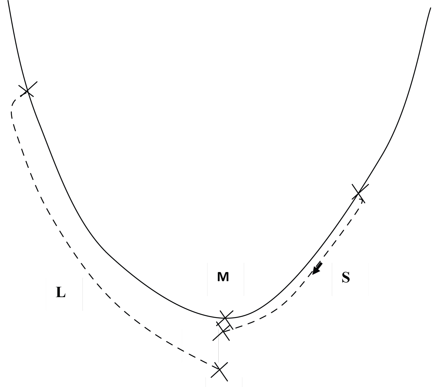
The present problem involves five control surface deflections, which could be used as coordinates in a five-dimensional space. The drag is a function of these five control surface deflections, and thus is a hyper-surface of dimension 4. The condition of pitch trim is represented by another hypersurface, and their intersection is a subspace of dimension 3. If the condition of constant lift is imposed as well, then the control surface deflections must lie on a subspace of dimension 2 (i.e. a surface) in the 5-dimensional space. The question of drag minimization subject to pitch trim and constant lift constraints then amounts to finding on this surface in 5-dimensional space the point where the drag is minimum. Alternatively, one could eliminate three deflections, and have the drag represented in 3-dimensions as a surface function only of two independent deflections. If this surface is convex, e.g. like a bowl, then there is only one local minimum, which is also the global minimum: the bottom of the bowl (point M in Figure 2). Starting from any initial condition, the optimization method imposes a "descent", which can only end at the "bottom" of the bowl. A "good" starting condition "close" to the bottom gives a short descent (path S in Figure 2), whereas a "poor" initial condition far from the "minimum" (path L) yields a longer descent. The final result should be the same, apart from an accumulation of errors which may be more significant for the "poor" initial condition, which requires more iterations. The question of accumulation of errors is relevant here, since the iterative procedure uses repeatedly second-order control derivatives, which may not be too accurate to start with.

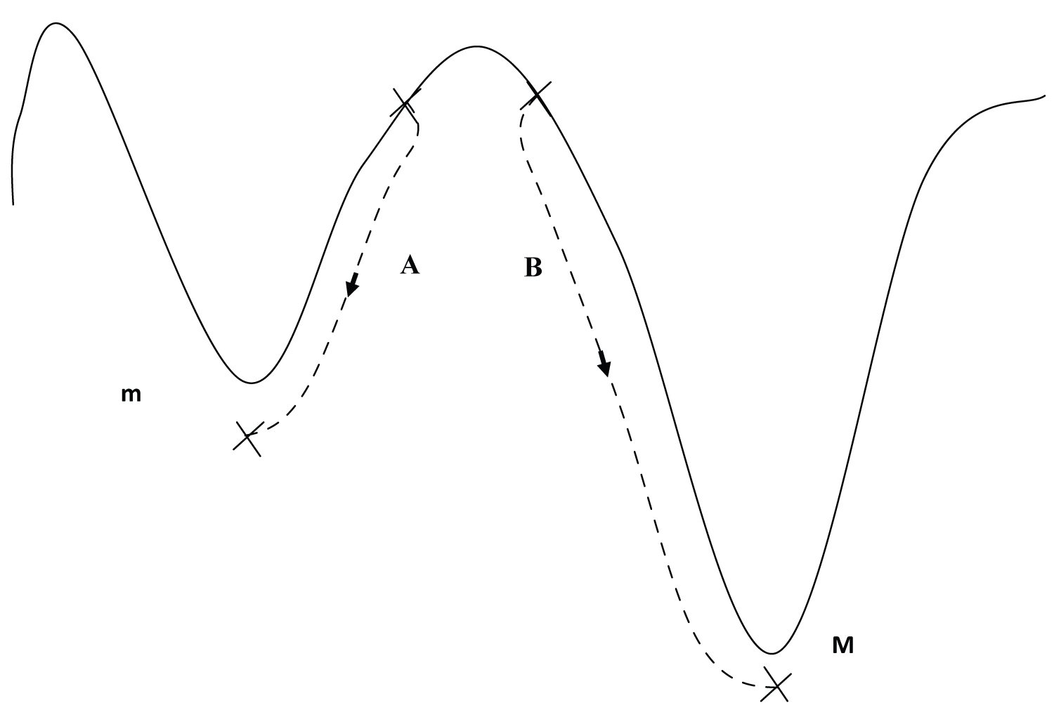
A more fundamental question is whether the drag surface, or to be more precise the surface associated with the intersection of drag, lift and pitching moment hypersurfaces is convex. If it is not, then it could have several valleys, i.e. several local minima (points M and m in Figure 3); depending on the starting point the optimization procedure could lead (path A and B in Figure 3) to different local minima, with no way to know if that particular local minimum is or not the global minimum, other than comparing the values at the two minima. In the case of the Figure 3 or the two local minima m > M the lowest or global minimum is M. However, starting in the left-hand bowl and reaching the local minimum m would give no indication of the existence of a lower global minimum M. To find the lowest global minimum the search may require considering all local bowls, as for the deepest valley (or highest peak) in a mountain range. If the drag derivatives had the same sign for all control surfaces, the corresponding hypersurface might be convex; however Table 5 shows that this is not the case, since the drag derivative for the ailerons has opposite sign to that for all other control surfaces. The lift and pitching moment derivatives have the same sign for all control surfaces; even if the lift and pitching moment hypersurface are convex there is no guarantee that their intersection is, let alone the triple intersection with a non-convex drag hypersurface.

In addition to the (i) Accumulation of iteration errors and; (ii) Possible existence of several local minima, it may also happen; (iii) That some minima be outside the limited range of variation of control deflections. In the latter case the "minimum" would be on the boundary of admissible deflections and might not be even a local minimum. The optimization method may be useful not just for the final optimal value. The very first iteration of the optimization procedure gave a useful indication of how some control surfaces should be deflected to minimize drag at constant pitching moment. However, a good understanding of the flight physics of the particular aircraft combination cannot be replaced by any method, even an optimal one.

Acknowledgements

This work was supported by FCT (Foundation for Science and Technology), through IDMEC (Institute of Mechanical Engineering), under LAETA, project UIDB/EMS/50022/2020. This work was started under the NACRE project of the European Union and benefited from comments of other partners in this activity.

References

1. McKinney L, Dollyhigh S (1970) Some trim drag considerations for maneuvering aircraft. AIAA 2nd Aircraft Design and Operations Meeting, USA, 1-10.
2. Goldstein S, Combs C (1974) Trimmed drag and maximum flight efficiency of aft tail and canard configurations. AIAA 12^th Aerospace Sciences Meeting, USA, 1-12.
3. McLaughlin M (1977) Calculations, and comparison with an ideal minimum, of trimmed drag for conventional and canard configurations having various levels of static stability. NASA Technical Note 1-22.
4. Kendall E (1984) The minimum induced drag, longitudinal trim and static longitudinal stability of two-surface and three-surface airplanes. AIAA 2nd Applied Aerodynamics Conference, USA, 1-10.
5. Ende R (1989) The effects of aft-loaded airfoils on aircraft trim drag. AIAA 27th Aerospace Sciences Meeting, USA, 1-9.
6. Campos LMBC, Marques JMG (2015) On the minimization of cruise drag due to pitch trim for a flying wing configuration. The CEAS Air and Space Conference 2015, Delft University of Technology, The Netherlands.
7. Rahman NU, Whidborne JF (2010) Propulsion and flight controls integration for a blended-wing-body transport aircraft. J Aircr 47: 895-903.
8. Haiqiang D, Xiongqing Y, Hailian Y, et al. (2015) Trim drag prediction for blendedwing-body UAV configuration. Trans Nanjing Univ Aeronaut Astronaut 32: 133-136.
9. Griffin BJ, Brown NA, Yoo SY (2011) Intelligent control for drag reduction on the X-48B vehicle. AIAA Guidance, Navigation and Control Conference, Portland, Oregon.
10. Durham W (1993) Constrained control allocation. J Guid Control Dyn 16: 717-725.
11. Harkegard O (2004) Dynamic control allocation using constrained quadratic programming. J Guid Control Dyn 27: 1028-1034.
12. Bolender MA, Doman DB (2005) Nonlinear control allocation using piecewise linear functions: A linear programming approach. J Guid Control Dyn 28: 558-562.
13. Jacobsen M (2006) Real time drag minimization using redundant control surfaces. Aerosp Sci Tech 10: 574-580.
14. Carlsson M, Cronander C (2005) Efficient roll control using distributed control surfaces and aeroeslastic effects. Aerosp Sci Tech 9: 143-150.
15. Bodson M (2011) Evaluation of optimization methods for control allocation. J Guid Control Dyn 34: 380-387.
16. Chambon E, Burlion L, Apkarian P (2017) Time-response shaping using output to input saturation transformation. International Journal of Control 91: 534-553.
17. Denieul Y, Bordeneuve J, Alazard D, et al. (2018) Multicontrol surface optimization for blended wing-body under handling quality constraints. Journal of Aircraft 55: 638-651.
18. Cook MV, de Castro HV (2004) The longitudinal flying qualities of a blended-wing body civil transport aircraft. Aeronaut J 108: 75-84.
19. Roysdon PF, Khalid M (2011) Blended-wing-body lateral-directional stability investigation using 6DOF simulation. AIAA Infotech at Aerospace Conference and Exhibit, St. Louis, Missouri.
20. Peterson T, Grant PR (2011) Handling qualities of a blended wing body aircraft. AIAA Atmospheric Flight Mechanics Conference, Portland, Oregon.
21. Jung DW, Lowenberg MH (2005) Stability and control assessment of a blended-wing body airliner configuration. AIAA Atmospheric Flight Mechanics Conference and Exhibit, San Francisco, California.
22. Cameron D, Princen N (2000) Control allocation challenges and requirements for the blended wing body. AIAA Guidance, Navigation and Control Conference and Exhibit, USA, 1-5.
23. Wildschek A, Stroscher F, Klimmek T, et al. (2010) Gust load alleviation on a large blended wing body airliner. 27th International Congress of the Aeronautical Sciences, Nice, France.
24. Waters SM, Voskuij M, Veldhuis LLM, et al. (2013) Control allocation performance for blended wing body aircraft and its impact on control surface design. Aerospace Science and Technology 29: 18-27.
25. Wildschek A, Bartosiewicz Z, Mozyrska D (2014) A multi-input multi-output adaptive feed-forward controller for vibration alleviation on a large blended wing body airliner. J Sound Vib 333: 3859-3880.
26. Kozek M, Schirrer A (2015) Modeling and control for a blended wing body aircraft - a case study. Advances in Industrial Control, Springer.
27. Peifeng L, Binqian Z, Yingchun C, et al. (2012) Aerodynamic design methodology for a blended wing body transport, Chinese Journal of Aeronautics 25: 508-516.
28. Campos L (2015) On physical aeroacoustics with some implications for low-noise aircraft design and airport operations. Aerospace 2: 17-90.
29. Huijts C, Voskuij M (2015) The impact of control allocation on trim drag of blended wing body aircraft. Aerospace Science and Technology 46: 72-81.
30. Okonkwo P, Smith H (2016) Review of evolving trends in blended wing body aircraft design. Progress in Aerospace Sciences 82: 1-23.
31. Kumar P, Khalid A (2017) Blended wing body propulsion system design. International Journal of Aviation, Aeronautics and Aerospace 4.
32. Ammar S, Legros C, Trépanier JY (2017) Conceptual design, performance and stability analysis of a 200 passengers blended wing body aircraft. Aerospace Science and Technology 71: 325-336.
33. Panagiotou P, Fotiadis-Karras S, Yakinthos K (2018) Conceptual design of a blended wing body MALE UAV. Aerospace Science and Technology 73: 32-47.
34. Dakka S, Johnson O (2019) Aerodynamic design and exploration of a blended wing body aircraft at subsonic speed. International Journal of Aviation, Aeronautics, and Aerospace 6: 17.
35. Kim H, Liou MF (2019) Flow simulation and drag decomposition study of N3-X hybrid wing-body configuration. Aerospace Science and Technology 85: 24-39.
36. Khan T (2019) Design and CFD analysis of a blended wing UAV (a conceptual design). J Aerosp Eng Mech 3: 156-160.
37. Wang G, Zhang M, Tao Y, et al. (2020) Research on analytical scaling method and scale effects for subscale flight test of blended wing body civil aircraft. Aerospace Science and Technology 106: 106114.
38. Footohi P, Bouskela A, Shkarayev S (2020) Aerodynamic characteristics of the blended-wing-body VTOL UAV. J Aerosp Eng Mech 4: 187-300.
39. Humphreys-Jennings C, Lappas I, Sovar DM (2020) Conceptual design, flying, and handling qualities assessment of a blended wing body (BWB) aircraft by using an engineering flight simulator. Aerospace 7: 51.
40. Jemitola P, Okonkwo P (2019) Review of structural issues in the design of a box wing aircraft. J Aerosp Eng Mech 3: 161-166.
41. Kalinowski Milosz (2017) Aero-structural optimization of joined-wing aircraft. Transactions on Aerospace Research 4: 48-63.
42. Pierre DA (1987) Optimization theory with applications. Dover Publications, USA.
43. Tavares LV, Correia NC (1984) Optimização linear e não-linear. Fundação Calouste Gulbenkian.
44. Goldberg DE (1989) Genetic algorithms. Addison-Wesley.
45. Woodhouse R (1810) History of the calculus of variations in the eighteenth century. Cambridge.
46. Bolza O (1904) Lectures on the calculus of variations. University of Chicago Press.
47. Bolza O (1909) Vorlesungen ueber variationsrechnung. AMS Chelsea Publishing.
48. Bliss GA (1925) Calculus of variations. Open Court.
49. Caratheodory L (1989) Calculus of variations. Teubner.
50. Seifert H, Theresfall W (1948) Variatiohrechnung in Grossen. Berlin.
51. Forsyth AR (1960) Calculus of variations. Cambridge University Press.
52. Weinstock R (1974) Calculus of variations. McGraw/Hill.
53. Fox C (1987) Calculus of variations. Oxford University Press.
54. Sagan H (1992) Calculus of variations. McGraw-Hill.
55. LMBC Campos, JMG Marques (2019) On the maximisation of control power in low-speed flight. The Aeronautical Journal 213: 1099-1121.
56. Lagrange JL (1960) Mécanique analitique. Académie des Sciences.
57. Hamilton WR (1830) Mechanics of particles. Royal Irish Academy.
58. Lanczos C (1962) The variational principles of mechanics. (2nd edn), University Press.
59. Pars LA (1960) Analytical dynamics. Heinemann.
60. Ter Haar D (1961) Elements of hamiltonian mechanics. North-Holland.
61. Luré L (1968) Mécanique analitique, Masson.
62. Gantmacher F (1975) Lectures on analytical mechanics, MIR Publishers.
63. Deriglazov A (2010) Classical mechanics. Springer.
64. Newton I (1934) Principia. Cambridge University, 1972, 5 vols, translation Dover.
65. Appel P (1919-1923) Traité de Mécanique Rationelle. 5 vols. 4éme édition, Gauthier-Villars 1900-1904.
66. Mathieu E (1878) Dynamique analytique. Gauthier-Villars.
67. Painlevé P, Platrier C (1929) Cours de Mécanique. Gauthier-Villars.
68. Routh EJ (1960) Dynamics of a particle. Dover Publisher, NY.
69. Routh EJ (1960) Dynamics of a system of rigid bodies. Dover Publisher, NY.
70. Hertz H (1956) The principles of mechanics. Dover Publisher, NY.
71. Ames JS, Murnaghan FD (1957) Theorical mechanics. Dover Publisher, NY.
72. Whittaker ET (1937) Analytical dynamic of particles and rigid bodies. (4th edn), Cambridge University Press.
73. Frank NH (1947) Mechanics. Greenwood Press.
74. Synge JL, Griffith B (1949) Principles of mechanics. McGraw-Hill, New York.
75. Cabannes H (1968) Mécanique. Dunod.
76. Hand LN, Finch JD (1998) Analytical Mechanics. Cambridge University Press.
77. Strauch D (2009) Classical mechanics. Springer.
78. Kuypers F (2016) Klassische Mechanik. Wiley-VCH, Berlin.