Active Flutter Suppression of Stochastic Airfoil with Uncertain Pitch Stiffness
Abstract
Flutter suppression of a typical airfoil with uncertain pitch stiffness by feedback control of its trailing-edge surface is analyzed. The pitch stiffness coefficient is modeled by a quadratic function of a bounded random variable with the bounded probability density function, thus the airfoil system becomes a stochastic structure depending on its random parameter. It is found that just like its deterministic counterpart the flutter suppression of stochastic airfoil system can also be realized by feedback control. In analysis the feedback controlled stochastic airfoil system is first reduced into its equivalent deterministic system by Gegenbauer polynomial approximation. The critical flutter speed of the stochastic airfoil system with control can be determined by Hopf-bifurcation point of its equivalent system. Then the problem of suppressing limit cycle oscillation of stochastic airfoil system by feedback control can be studied numerically via the equivalent deterministic system. Numerical results show that the critical flutter speeds of a stochastic airfoil system can be reasonably lifted by properly control its trailing-edge surface. And this kind of feedback control is robust.
Keywords
Stochastic airfoil, Flutter suppression, Feedback control, Robust control, Hopf-bifurcation, Limit cycle oscillation, λ-PDF, Gegenbauer polynomial approximation
Nomenclature
ξη: Bounded Random Variable; pλ(ξ): Probability Density Function; λ: Parameter; τ(λ): Gamma Function; : Gegenbauer Polynomials; (λ)k: Pochhammer Symbol; h: Plunge Displacement; θ: Pitch Angle; t: Time; m: Mass about the Elastic Axis per Unit Span; Iθ: Moment of Inertia about the Elastic Axis per Unit Span; xθ: Non-Dimensional Distance Between Center of Gravity and the Elastic Axis; ch,cθ: Viscous Damping Coefficients; kh: Linear Plunge Stiffness; kθ(θ): Nonlinear Pitch Stiffness; b: Semi-Chord Length of the Airfoil; L: Aerodynamic Lift; M: Aerodynamic Moment; ρ: Air Density; U: Speed; : Lift Coefficient per Unit Angle of Attack; : Lift Moment per Unit Angle of Attack; : Lift Coefficient per Unit Angle of Attack of the Control Surface; : Lift Moment per Unit Angle of Attack of the Control Surface; ab: Non-dimensional Distance Between the Elastic Axis and the Middle Point of Chord; ϕ: Angle of Attack; δ1, δ2: Control Parameters; kθ k'θ: Random Parameters.
Introduction
Aircraft wing flutter is a kind of self-excited oscillation resulting from interactions of inertia, elastic, and aerodynamic forces on the structure [1]. Wing flutter may deteriorate structural integrity and even lead to failure of wings. Thus, the prediction of flutter onset and the active suppression of flutter are of the utmost importance in aircraft design.
In the past few decades as a main topic of nonlinear aero-elasticity the studies on mechanism of flutter and various strategies for suppressing flutter have been paid on a great amount of attention. An active flutter suppression strategy for a nonlinear airfoil was examined by Block and Strganac [2], which effectively extends the stable flight region. Based on a back-stepping design technique, Xing and Singh suggested an adaptive controller for the control of an aero-elastic system by output feedback [3]. An analytical and experimental study of a control surface with distributed piezoelectric actuators for active flutter suppression of a wing model was reported by Chen, et al. [4], whose test results show that compared with the open loop system, the close loop system increases its critical flutter speed by 12%. Analytical and experimental studies on active flutter suppression of a wing section by both the leading and the trailing surfaces were reported by Platanitis and Strganac [5], where uncertainty in the nonlinear pitch stiffness was examined. A semi-active flutter suppression strategy for wing section through trailing edge surface control was suggested by Sun, Wen and Hu [6] by using an actuator equipped with Magneto-Rheological (MR) damper. Their simulation results show that the on-off control of MR damper can increase the critical flutter speed by 17% or so.
However, most of the above-mentioned works are limited to deterministic airfoil model only. In fact, some parameters of an airfoil system may be uncertain, for example the pitch stiffness. For the sake of simplification and emphasis on the main effect of the deterministic structure, these uncertainties used to be neglected in analysis. Yet it is more reasonable to model an uncertain physical parameter as a random variable with a given probability density function (λ-PDF for short). Thus, the system considered becomes a stochastic system, whose characteristics depend upon the random variable. And the dynamical behavior in a nonlinear stochastic system is much more complicated than in the corresponding deterministic system. One has to deal with the problem of stochastic bifurcation and even stochastic chaos.
A current mathematical tool to solve the dynamical problem of a stochastic system is the orthogonal polynomial approximation, which is forwarded by Spanos and Ghanem [7], and further developed later on by Li [8]. In view of stochastic structures with bounded random parameters Fang, et al. first used Chebyshev polynomial approximation to solve the evolutionary random response problem of a stochastic system with random variables of an arch-like PDF [9]. Later on Gegenbauer polynomial approximation was suggested by Fang, et al. to solve the dynamical problem of stochastic systems with bounded random variables of λ-PDF [10-15], including the problem of stochastic bifurcation and stochastic chaos and its control or synchronization.
In this paper Gegenbauer polynomial approximation is used to analyze the active flutter suppression of an airfoil system with bounded random parameter of λ-PDF. The stochastic airfoil system is first transformed into its equivalent deterministic system. And the critical flutter speed of the stochastic airfoil system with control can be determined by the Hopf-bifurcation point of its equivalent system. Then the active suppression of limit cycle oscillation of the stochastic airfoil system can be studied through numerical simulations of the equivalent system. Simulation results show that the critical flutter speed of a stochastic airfoil system can be reasonably lifted by proper control of its trailing-edge surface.
λ-PDF and Gegenbauer Polynomial Functions
The probability density functions of a broad type of bounded random variable ξ can be modeled by the so-called λ-PDF, which can be expressed as follows
where λ ≥ 0 is a fixed parameter, and ρλ is a normalizing constant expressed by
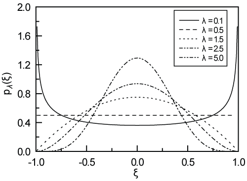
where τ(λ) is a Gamma function. The graphs of λ-PDF for different values of λ can be shown as Figure 1.
One can see that when λ = 0, λ-PDF is a pitfall-like distribution
When λ = 0.5, λ-PDF is a uniform distribution
And when λ = 1, λ-PDF is an arch-like distribution
One can also see that any bounded random parameter symmetrically defined on [-1, 1], with a mono-peak (or mono-valley) might be modeled approximately by ξ with one of the λ-PDF's most close to it. In addition even some un-symmetrically bounded random parameters can also be approximately modelled by certain polynomial functions of ξ [15].
It is well-known that in orthogonal polynomial approximation the choice of orthogonal basis depends on the probability density function of the random parameter considered. For example, Hermite polynomials for Gaussian random parameter, Legendre polynomials for bounded uniformly distributed random parameter, and so on. As for random parameters with λ-PDF, Gegenbauer polynomials are the unique right choice for orthogonal basis. The first few Gegenbauer polynomials are as follows.
The orthogonal relationships of Gegenbauer polynomials may be expressed as
Where
The first and the second order recurrent formulas for Gegenbauer polynomials are expressed as [15]
and
where
Equation (7) implies a kind of weighted averaging property with λ-PDF as a weighting function. Owing to the orthogonal relationships of Gegenbauer polynomials, any f(ξ) ⊂ L2, defined on [-1, 1] can be expressed as a series of , namely
where
It is worth noting here that Eq. (12) is valid only for taking the sum over infinite number of items. If in practice only a limited number of items are taken in this equation, the result is merely an approximation with a minimal mean square residual.
Dynamic Equation of a Stochastic Airfoil System
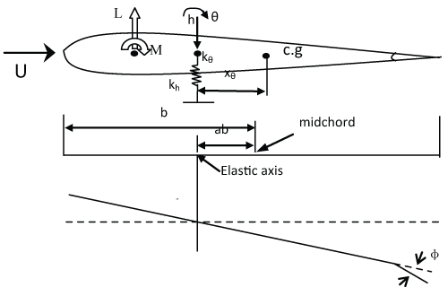
A nonlinear stochastic airfoil system permitting plunge h and pitch θ motion about the elastic axis, and equipped with a trailing-edge control surface is shown in Figure 2. The dynamical equation of the system, neglecting control surface dynamics, may be described as
where h and θ stand for system responses; an overhead dot on h or θ denotes d/dt , and t is the time ; m and Iθ are mass and moment of inertia about the elastic axis per unit span, respectively; xθ is non-dimensional distance between center of gravity and the elastic axis; ch and cθ are viscous damping coefficients for plunge and pitch motion respectively; kh and kθ(θ) are linear plunge stiffness and nonlinear pitch stiffness respectively; b is the semi-chord length of the airfoil; and L and M are quasi-steady aerodynamic lift and moment, which can be approximately expressed as
where ρ and U represent air density and the speed of coming incompressible flow respectively; , are coefficient of lift and moment per unit angle of attack of the airfoil; , are coefficient of lift and moment per unit angle of attack of the control surface; ab is the non-dimensional distance between the elastic axis and the middle point of chord; and ϕ is the angle of attack of the control surface to carry out the feedback control law.
It is well-known that for a conventional airfoil system the state feedback control of its trailing edge surface is an effective way to suppress airfoil flutter. To illustrate this flutter suppression strategy applies as well to a stochastic airfoil system, we simply use the proportional feedback control law, namely,
Where δ1, δ2 are independent control parameters.
In general the coefficient of nonlinear pitch stiffness kθ(θ) is difficult to obtain analytically. One could only find its approximate expression through curve fitting the experimental data. Now we assume kθ(θ) may be expressed in the form
Where kθ and k'θ are to be determined yet. Since there is always some uncertainty in measuring and manufacturing, we would rather take kθ and k'θ as random parameters. Without losing generality, we assume that they can be modeled by a quadratic function of a bounded random variable ξ with a given λ-PDF, namely
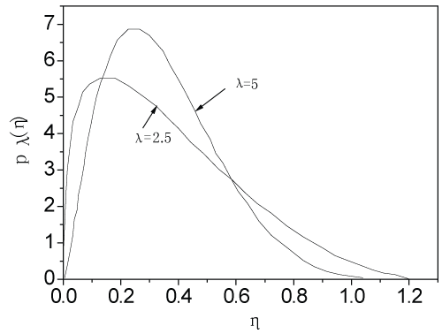
Where kθ, k'θ, σ1, σ2, σ'1, σ'2 are properly selected deterministic constants. For different values of these constants, kθ, k'θ may have different probability distributions. For example, let η = kθ/kθ, σ1 = 0.2, and σ2 = 0.1, then the probability density function of η can be shown as Figure 3. One can see that pλ(η) even can be un-symmetric. Substituting equations (15) - (18) into Eq. (14), we have the following dynamical equation for the stochastic airfoil system
Where ,
,
This is what we need the dynamic equation of a 2-DOF nonlinear stochastic airfoil system with feedback control, which can be further processed by the Gegenbauer polynomial approximation.
Gagenbauer Polynomial Approximation for a Stochastic Airfoil System
Since the system (19) itself depending upon a bounded random parameter ξ, the response of the system should be a function of both t and ξ, namely
In Gegenbauer polynomial approximation these responses can be approximated by
where represents the lth order Gegenbauer polynomial, and N stands for the highest order we have taken. When N → ∞, and are exact solutions of Eq. (19), otherwise they are just approximate solutions. In practice we can choose a proper N to meet the required accuracy.
Substituting Eq. (21) into Eq. (19), we have
By using the recurrent formulas of Gegenbauer polynomials, Eq. (9) - Eq. (10), we can eliminate the random variables explicitly appearing in the second equation of Eq. (22). Thus, the linear term can be rewritten as
While deriving Eq. (23), it is assumed that θl(t) = 0,when l > N or l < 0, which is also valid in the following derivation.
The nonlinear term in Eq. (22) can be expanded as
By Eq. (6) the product can be rewritten as
Where
Where can be written as in which (λ)k is the Pochhammer symbol, which stands for
It is worth noting that in Eq. (26) we have , when m > n. By Eq. (6) the term [(ξ - 1)/2]m can be expressed as a linear combination of as
where
By substituting Eq. (27) into Eq. (25), the product can be expressed as linear combinations of individual Gegenbauer polynomials, namely
where
Substituting Eq. (29) into Eq. (24), we have
Where
Similarly, by the recurrent formulas Eq. (9) - Eq. (10), the nonlinear term can be reduced into
Substituting Eq. (23) and Eq. (33) into Eq. (22), we have
Multiplying , (i = 0,1,….,N) onto both sides of Eq. (34) in sequence, then taking expectations with respect to ξ, owing to the orthogonality relationships of Gegenbauer polynomials, we finally obtain
Now Eq. (35) is a deterministic nonlinear one obtained through some weighted averaging by Gegenbauer polynomial approximation on the stochastic airfoil system with feedback control. We call it an equivalent deterministic system, which plays a significant role in the following analysis. Since Eq. (35) is deterministic, it can be solved by any available effective conventional theory or method, including Runge-Kutta method, MATLAB, MAPLE and so on. Once hi(t), θi(t) (i = 0~N) are obtained through Eq. (35), the approximate stochastic responses of the stochastic airfoil system can be readily obtained through Eq. (21), namely
And the ensemble averaging responses are simply as
For any sample random variable , the sample responses of the stochastic system are as
Critical Flutter Speed of Stochastic Airfoil System
By introducing the following state variables
the equivalent deterministic system can be rewritten into a system of first order differential equations
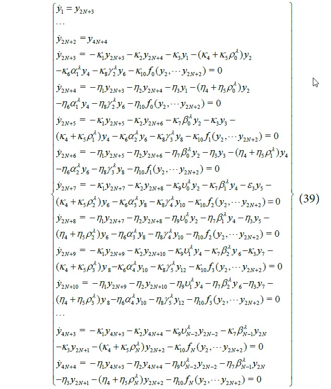
where
Eq. (39) can be written in short as
The critical flutter speed can be determined by the Hopf-bifurcation point of Eq. (40), which is the transition point of equilibrium solution into self-excited oscillatory solution [16]. The Hopf-bifurcation point of Eq. (40) can be determined as follows.
Let the equilibrium solution of Eq. (40) be YE, then the transient solution in its neighborhood may be assumed as
where ε is an infinitesimal, and P = P1 + iP2 is a complex eigenvector with respect to the imaginary eigenvalue iω. Substituting Eq. (41) into Eq. (40), and expanding it into a Taylor series around YE, we have
At the equilibrium point YE, we have
Substituting Eq. (43) into Eq. (42), and neglecting the second and higher order terms, we have
Then inserting P = P1 + iP2 into Eq. (44) and letting the imaginary and the real parts of the equation equal zero, we have
To guarantee Eq. (45) having unique solutions P1 and P2, we need the following additional restriction equations
where q is a constant vector [16]. Combining Eq. (43), Eq. (45) and Eq. (46) into one, we have the following equation
Eq. (47) can be solved by the Newtonian iterative method.
Numerical Results and Discussions
The effectiveness of the proposed flutter suppression strategy for a stochastic airfoil system can be shown through illustrative numerical examples. In calculation the deterministic data of airfoil system are taken as follows [17]
a = -0.6, b = 0.135 m, kh = 284404 N/m, ch = 27.43 Ns/m, , , , , , , ,
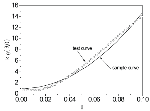
The pitch stiffness coefficients Kθ, K'θ, can be obtained through curve-fitting of experimental data. Here we take Kθ = 2.82, K'θ = 1215. Figure 4 shows the variation of a sample kθ(θ, 0) of the stochastic stiffness coefficient kθ(θ, ξ) against θ, compared with test results cited from Ref [17]. One can see that the sample curve kθ(θ, 0) is a good approximation of the test data, as long as θ is small enough. The other coefficients σ1, σ2, σ'1 and σ'2 in Eq. (18) are taken several different values for comparative study.
In analysis the highest order of the Gegenbauer polynomial we take is N = 6, and λ = 1.5.
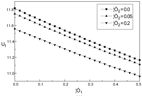
Now we are going to look into the influence of random pitch stiffness on the critical flutter speed Uf of the stochastic airfoil without feedback control, i.e. when δ1 = 0.0, δ2 = 0.0. In fact, we can obtain the critical flutter speed Uf of the stochastic airfoil without feedback control by solving equation (47). For simplicity in calculation we take σ'1 and σ'2 as fixed parameters, and let σ'1 = 0.1 and σ'2 = 0.1; and properly adjust the values of σ1 and σ2. The numerical results for variation of critical flutter speed Uf against σ1 and σ2 are shown in Figure 5. One can see that as σ1 and σ2 increase, the critical flutter speed Uf decreases monotonously. That is to say the increase of σ1 and σ2 always brings about negative influence on the critical flutter speed of the stochastic airfoil system.
Then, we look into the effect of feedback control on suppressing flutter of the stochastic airfoil system under coming flow with different airspeeds U. In this case we take
and properly adjust the values of control parameters δ1 and δ2 while carrying out numerical simulations to observe the effect of flutter suppression by feedback control. The simulation results are shown in Figure 6, Figure 7, Figure 8, Figure 9 and Figure 10 respectively. In Figure 5 one can find the critical flutter speed of the stochastic airfoil system without control under the condition (48) is Uf = 11.61 m/s, which will be used as a reference later.
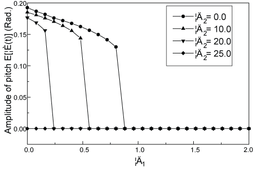
Under the condition U = 13 m/s, variations of limit cycle oscillation for pitch motion against δ1 and δ2 are shown in Figure 6. It can be seen that for δ2 = 25.0 the limit cycle oscillation can be suppressed at all for whatever δ1 not less than zero; while for δ2 = 20.0 , 10.0 , or 0.0, the limit cycle oscillation can only be suppressed at all for δ1 > 0.24 , 0.56 , or 0.88 respectively.
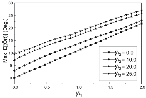
Figure 7 shows the variation of the maximum angle of attack of the control surface against δ1 and δ2 under U = 13 m/s. It can be seen that the greater the δ1 and δ2 are, the larger the maximum angle of attack of the control surface.
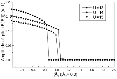
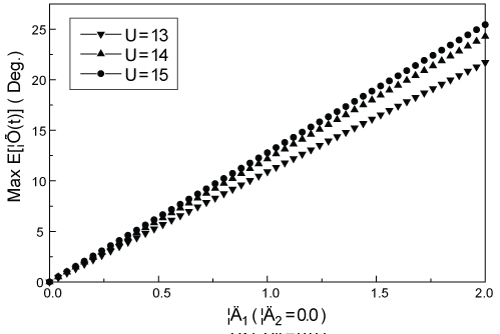
Figure 8 shows the variation of limit cycle oscillation against δ1 under different speeds of coming flow. One can see that as the speed of coming flow increases, the minimum δ1 required for fully suppressing limit cycle oscillation becomes greater. For U = 13, 14 or 15 m/s, the minimum δ1 required is 0.88, 1.04 or 1.2 respectively.
Figure 9 shows the variation of the maximum angle of attack of the control surface under different speeds of coming flow. One can see that for a same value of δ1 the greater the speed of coming flow, the larger the maximum angle of attack of the control surface. For example, for δ1= 1.2 and U = 13, 14, or 15m/s, the maximum angle of attack of the control surface is 13º, 14.6º or 15.3º respectively.
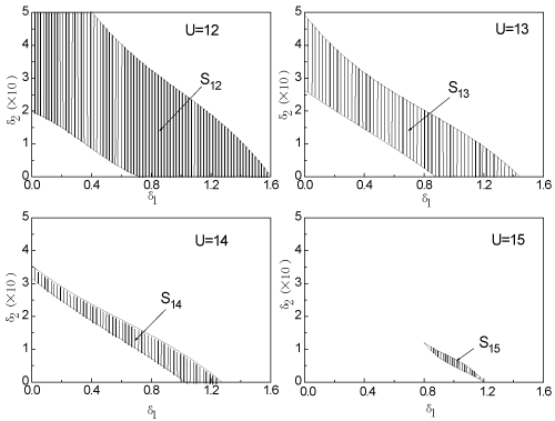
It is worth mentioning here that while modeling the airfoil system we have not neglected the dynamics of the control surface itself, nor have we introduced any executor for realizing the required angle of attack, ϕ, of the control surface. To remedy this shortcoming in analysis, all what we can do for drawing reasonable conclusions from our analysis is to set some threshold for the maximum angle of attack of the control surface, i.e. |ϕ| ≤ ϕ. Thus, this restriction determines the upper limits of δ1 and δ2. On the other hand the lower limits of δ1 and δ2 can be determined by the condition of totally suppressing the limit cycle oscillation, i.e., |E[θ(t)]| ≤ ε', where ε' is a given small positive number. In this paper we take ϕ = 15º and ε' = 0.0001, and determine the upper and lower limits for δ1 and δ2 in this way. Figure 10 shows the available domains S12, S13, S14 and S15 for δ1 and δ2 corresponding to U = 12, 13, 14 and 15 m/s respectively. It can be seen that S15 ⊂ S14 ⊂ S13 ⊂ S12, namely as the speed of coming flow increases, the available domain of δ1 and δ2 becomes smaller and smaller. In fact, when U = 15 m/s, the available domain for δ1 and δ2 becomes too narrow that the feedback control through trailing-edge surface can hardly suppress flutter of the airfoil system any longer. However, if we choose δ1 = 1.1 and δ1 = 0.3 in S14 as working point of the control law, there is still enough room for deviation of δ1 and δ2. And in a conservative way, even if U = 14 m/s is taken as the critical flutter speed of the controlled airfoil system, it is 20% higher than that (= 11.61m/s) of the stochastic airfoil without control.
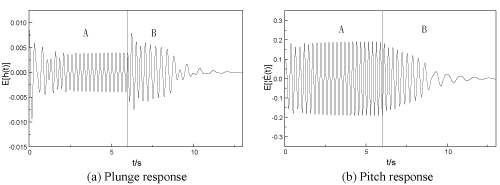
To illustrate further the function of feedback control on suppression of flutter, Figure 11 shows the time history of the ensemble average response with or without feedback control under the conditions that the speed of coming fluid is taken as U = 13 m/s and the initial state conditions are taken as follows.
At first the response of the open loop system without control presents a limit cycle oscillation; while after the feedback control with δ1 = 1.0, δ1 = 0.0 turns on at t = 6 s, the transition of motion begins and the response of the close loop system soon drops down to the equilibrium position.
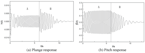
What shown in Figure 11 clearly illustrates the process of flutter suppression for the ensemble averaging response of the airfoil system. It can be shown that if the ensemble averaging response gets suppressed, so does its every sample response. For example, for , δ1 = 1.0, δ1 = 0.0, the time history of sample response of the open loop system and the close loop system is shown in Figure 12. One can see that the suppression of flutter for the sample response of stochastic airfoil system also works. In this sense, the active flutter suppression strategy for stochastic airfoil system has the ensemble effect. In other word, the active flutter suppression strategy works well within the whole define domain of the random variable. In this sense the suggested feedback control of stochastic airfoil system is robust.
Conclusions
It may be the first time to analyze the problem of feedback control of a stochastic airfoil system with bounded random parameters. The Gegenbauer polynomial approximation bridges the gap between the stochastic system and the available method for deterministic analysis, and applies effectively to a nonlinear stochastic airfoil system with feedback control as well. Through the Hopf-bifurcation analysis and the numerical simulation results of the equivalent deterministic system, it is shown that the suggested active flutter suppression strategy for a stochastic airfoil system really works well. And the feedback control in this case is in robust sense.
References
- Dowell EH, Edward J, Strganac TW (2003) Nonlinear Aeroelasticity. Journal of Aircraft 40: 857-874.
- Block JJ, Strganac TW (1998) Applied active control for a nonlinear aero-elastic structure. Journal of Guidance, Control and Dynamics 21: 838-845
- Xing WH, Singh SN (2000) Adaptive output feedback control of a nonlinear aero-elastic structure. Journal of Guidance, Control and Dynamics 23: 1109-1116.
- Chen WM, Guan D, Li M (2002) Flutter suppression using distributed piezo-electric actuator. Acta Mechanica Sinica 34: 756-763.
- Platanitis G, Strganac TW (2004) Control of a nonlinear wing section using leading and trailing edge surfaces. Journal of Guidance, Control and Dynamics 27: 52-58.
- Sun W, Wen JS, Hu HY (2004) Semi-Active flutter suppression for wing aileron with framework system. Journal of Nanjing University of Aeronautics & Astronautics 36: 422-426.
- Spanos PD, Ghanem RG (1989) Stochastic finite element expansion for random media. J Eng Mech 115: 1035-1053.
- Li J (1996) The expanded order system method of combined random vibration analysis. Acta Mechanica Sinica 28: 66-75.
- Fang T, Leng XL, Song CQ (2003) Chebyshev polynomial approximation for dynamical response problem of random system. Journal of Sound and Vibration 226: 198-206.
- Fang T, Leng XL, Ma XP, et al. (2004) λ-PDF and Gegengbauer polynomial approximation for dynamic response problems of random structures. Acta Mechanica Sinica 20: 292-298.
- Ma XP, Leng XL, Meng G, et al. (2004) Evolutionary earthquake response of uncertain structures with bounded random parameter. Probabilistic Engineering Mechanics 19: 239-246.
- Leng XL, Wu CL, Ma XP, et al. (2005) Bifurcation and chaos analysis of stochastic Duffing system under harmonic excitations. Nonlinear Dynamics 42: 185-198.
- Wu C, Lei Y, Fang T (2006) Stochastic chaos in a Duffing oscillator and its control. Chaos, Solitons & Fractals 27: 459-469.
- Wu CL, Rong HW, Fang T (2007) Chaos synchronization of two stochastic Duffing oscillators by feedback control. Chaos, Solitons & Fractals 32: 1201-1207.
- Wu CL, Ma XP, Fang T (2006) A complementary note on Gegenbauer polynomial approximation for random response problem of stochastic structure. Probabilistic Engineering Mechanics 21: 410-419.
- Griewank A, Reddien G (1983) The Calculation of Hopf Points by a Direct Method. IMA Journal of Numerical Analysis 3: 295-303.
- Ko J, Strganac TW, Kurdila AJ (1998) Nonlinear adaptive control of an aeroelastic system via geometric methods. AIAA Paper 98-1795.
Corresponding Author
Wu Cunli, Department 10, Aircraft Strength Research Institute of China, 710065, P.Box. 86, Xi'an, P.R. China, Tel: +86-29-88268026.
Copyright
© 2017 Cunli W, et al. This is an open-access article distributed under the terms of the Creative Commons Attribution License, which permits unrestricted use, distribution, and reproduction in any medium, provided the original author and source are credited.