Dynamic Response and Vibration Control of a Planar Tensegrity Beam under El Centro Seismic Excitation

Abstract

Tensegrity systems are mechanical structures made of struts in compression, kept in stable equilibrium by a network of cables in tension, they are a class of mechanical structures which are highly controllable. This paper describes the dynamic response and vibration control of Tensegrity systems under seismic excitation. After giving the dynamic model of Tensegrity system under seismic excitation, the optimal control theory Linear Quadratic Regulator (LQR) algorithm is introduced as a possible method to be used in designing active control. A planar Tensegrity beam comprising of two modules, with pretension 30 cables and 8 struts with piezoelectric actuators, is optimized. The results show that vibration amplitudes of members are successfully reduced by such a kind of approach.

Keywords

Tensegrity systems, Dynamic response, Vibration control, Seismic excitation, LQR algorithm

Introduction

Tensegrity systems are spatial, reticulated and lightweight structures that have been known for almost half a century. The makeup of these structures consists of compressed struts and tensioned cables [1,2]. The tensioned cables of the structure are self-stressed such that the entire system could be provided stable equilibrium before any external loads is added, including gravitational. Due to this characteristic, systems will be composed of a network of cable members joined by discontinuous and limited compression members. A widely acknowledged definition has been proposed by Motro [3]. "A Tensegrity is a system in stable self-equilibrated state comprising a discontinuous set of compressed components inside a continuum of tensioned components". These smart structures have a large number of potential applications, for the benefit of systems which need, for instance, a small transportation, tunable stiffness properties, active vibration damping and deployment or configuration control. Because of these kinds of potential applications, since Tensegrity systems appeared in the early 1950s, they have been a matter of surprise and fascination. Until now, the concept of Tensegrity has been applied range from architecture, aerospace, civil engineering to biological fields.

Compared to the research related to geometry, form finding and architecture of Tensegrity structure, only few studies focused on the dynamic behavior. Motro, et al. [4] performed dynamic experimental and numerical work on a Tensegrity structure composed of 3 bars and 9 struts. They showed that a linearized dynamic model around an equilibrium configuration provides a good approximation of the nonlinear behavior of simple Tensegrity structure. Ben Kahla, et al. [5] proposed a numerical procedure for nonlinear dynamic analysis of Tensegrity systems. Oppenheim and Williams [6] concluded that friction in the rotational joints of the structure is a more important source of damping than the damping in tendons. Oppenheim and Williams [7] examined the dynamic behavior of a simple elastic Tensegrity structure, and found that the natural damping of the Tensegrity elements is poorly mobilized duo to the existence of infinitesimal mechanisms. Sultan, et al. [8] derived linearized dynamic models for two classes of Tensegrity structures and showed that the modal dynamic range generally increases with the pretension. Masic and Skelton [9] utilized a linearized dynamic model to enhance the dynamic control performance of a Tensegrity structure. Tan and Pellegrino [10] investigated the nonlinear vibration of a cable-stiffened pantographic deployable structure and showed that the system resonant frequencies are related to the level of active cable pretension.

Control of Tensegrity systems has been a topic of research since the middle of the 1990s. As is mentioned above, Tensegrity structures are a class of mechanical structures which are highly controllable. Skelton, et al. [11] concluded that as only small amounts of energy are needed to change the shape of Tensegrity structures, they are advantageous for active control. Djouadi, et al. [12] described the active vibration control of class 2 Tensegrity structure undergoing large deformations by use of an instantaneous optimal control scheme coupled with a finite element analysis based on geometric nonlinearity. Sultan [13] presented a formulation of Tensegrity active control and illustrated it with the example of an aircraft motion simulator. Kanchana saratool and Williamson [14] proposed a nonlinear constrained particle model of a Tensegrity platform, they used this model to study Tensegrity feedback shape control and developed a path tracking algorithm using neural networks. Van de Wijdeven and de Jager [15] studied an example of 2D Tensegrity vibration and shape control. Bel Hadj Ali and Smith [16] described the dynamic behavior and vibration control of a full-scale active Tensegrity structure. All these studies obtained results mainly from numerical simulation of small, simple, and symmetric Tensegrity models. Nelson [17] investigated the vibration control of a Tensegrity beam under sinusoidal excitation in her doctoral dissertation.

On the other hand, utilization of discrete piezoelectric actuators has been shown to be a viable concept for vibration control in various works. Crawley and de Luis [18] proposed an analytical solution for a static case including various actuator geometries. They suggested that discrete piezoelectric actuators could be considered in vibration control of some modes of vibration flexible structures. Kalaycioglu and Misra [19] used a dynamic modeling technique for vibration control of plate structures by utilizing PZT patches. The technique incorporates geometrical and mechanical properties of the actuator with the structures on which they mounted. Suleman [20] presented the effectiveness of the piezoceramic sensor and actuators on the suppression of vibrations on an experimental wing due to gust loading. They showed the feasibility of application of the smart structures in the suppression of vibrations due to the gust loading on the smart wing.

Researchers have recently focused their attentions on seismic-response-controlled structures which are being accepted as a fresh concept that can respond to the needs of a society in the new century. Kobori [21] proposed the concept of seismic-response-controlled structures and suggested this as the future direction on research. Raja and Narayanan [22] discussed the vibration control of Tensegrity structures under stationary and non stationary random excitation using H₂ and H∞ controller. Chen, et al. [23] described a design method for the H∞ state-feedback controller in finite frequency range to attenuate seismic-excited building vibration.

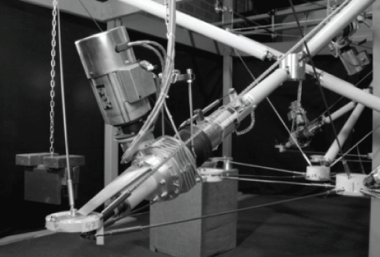
This paper proposed an idea of utilizing discrete piezoelectric actuators (Figure 1) in Tensegrity systems in order to create structures which can adapt to maintain stability, serviceability and reliability requirements. The importance of this paper is the introduction of concept (seismic-response-controlled structures) to Tensegrity systems, meanwhile, optimal active control of Tensegrity systems is considered by optimizing the structure and controller simultaneously. Based on the dynamic model of Tensegrity system under seismic excitation, the shape of structure is optimized with the node displacement as the design variable and the force generated by piezoelectric actuators is also considered as that mentioned in the work of Raja and Narayanan [24]. Numerical example shows that the LQR control is suitable for the vibration control of Tensegrity systems under seismic excitation.

Dynamic Model under Seismic Excitation

In this section, a linearized dynamic model written around an equilibrium configuration will be used to describe the dynamic behavior of the active Tensegrity system under seismic excitation. The linearized differential equation at a pre-stressed configuration can be written as:

$$\widehat{M}\widehat{\ddot{x}}(t)+\widehat{C}\widehat{\dot{x}}(t)+{\widehat{K}}_b\widehat{x}(t)=-\widehat{M}{\widehat{\ddot{x}}}_g(t)=\widehat{F}(t)(1)$$

Here $\stackrel{\wedge }{M}$, $\stackrel{\wedge }{C}$ and ${\stackrel{\wedge }{K}}_b$ refers to the mass, damping and stiffness matrix, respectively, $\stackrel{\wedge }{F}\left(t\right)$ represents the seismic excitation, vector $\stackrel{\wedge }{x}$, $\stackrel{\wedge }{\dot{x}}$ and $\stackrel{\wedge }{\ddot{x}}$ represents the vector of nodal displacement, velocity and acceleration, respectively, ${\stackrel{\wedge }{\ddot{x}}}_g$ refers to the ground acceleration caused by earthquake.

The tangent stiffness matrix ${\stackrel{\wedge }{K}}_b$ is decomposed into the linear stiffness matrix ${\widehat{K}}_{LA}$, commonly used for small-deformation truss analysis, and the geometrical stiffness included ${\widehat{K}}_{NL}$ by self-stress [3].

$${\stackrel{\wedge }{K}}_{{}_b}={\stackrel{\wedge }{K}}_{{}_{LA}}+{\stackrel{\wedge }{K}}_{{}_{NL}}(2)$$

For the development of a finite element model of the Tensegrity system, each element in the structure is characterized by the following mass and stiffness matrices [25]:

$${\widehat{K}}_{LA}=\left(\frac{EA}{L}\right)\cdot \left[\begin{array}{cc}{I}_0& -I_0\\ -I_0& I_0\end{array}\right](3)$$

$${\widehat{K}}_{NL}=\left(\frac{T}{L}\right)\cdot \left[\begin{array}{cc}{I}_3& -I_3\\ -I_3& I_3\end{array}\right]=q\cdot \left[\begin{array}{cc}{I}_3& -I_3\\ -I_3& I_3\end{array}\right](4)$$

$$\widehat{M}=\left(\frac{m}{6}\right)\cdot \left[\begin{array}{cc}2I_3& -I_3\\ -I_3& 2I_3\end{array}\right](5)$$

Where: $I_0=\left[\begin{array}{l}100\\ 000\\ 000\end{array}\right],I_3=\left[\begin{array}{l}100\\ 010\\ 001\end{array}\right]$

here, defining q = T/L as the force density coefficient for the member, E refers to the elastic modulus, A refers to the member area, L refers to the length of the member and T refers to the axial load. So the global mass and stiffness matrices M and K_b can be obtained by adding up contributions from the individual elements expressed in a global coordinate system.

By neglecting the damping matrix and the seismic excitation in Equation (1), the modal analysis of the Tensegrity system can be conducted as follows:

$$[K_b-{\omega }^{2}M]\overline{x}\left(t\right)=0(6)$$

Where ω refers to the natural frequency.

defining n as the degree of freedom of a Tensegrity system, the above equation gives the natural frequency ω_r (r = 1 : n) and the modal matrix $\varphi$, modal masses as well as modal loading can be determined by Equation (7) and Equation (8):

$$M_r={\varphi }_{r}M{\varphi }_r={\displaystyle \sum _{i-1}^n{m}_i}{\varphi }_{ir}^2(7)$$

$$F_r={\varphi }_r^{T}f=-{\ddot{x}}_g{\displaystyle \sum _{i-1}^n{m}_i}{\varphi }_{ir}(8)$$

defining yr (t) as the generalized coordinates, the uncoupled equations of motion for each mode can be formulated as:

$$\begin{array}{l}{\ddot{y}}_r\left(t\right)+2{\xi }_r{\omega }_r{\dot{y}}_r\left(t\right)+{\omega }_r^2{y}_r\left(t\right)=P_r/M_r=-{\ddot{x}}_g\left(t\right).\left({\displaystyle \sum _{i-1}^n{m}_i}{\varphi }_{ir}/{\displaystyle \sum _{i-1}^n{m}_i}{\varphi }_{ir}^2\right)(9)\\ \end{array}$$

here ξr refers to the damping ratio corresponding to the mode of r .

The maximum displacement of each mode can be computed as a function of the maximum of acceleration:

$$S_r=\frac{1}{{\omega }_r^2}{\ddot{S}}_r\frac{{\displaystyle \sum _{i-1}^n{m}_i}{\varphi }_{ir}}{{\displaystyle \sum _{i-1}^n{m}_i}{\varphi }_{ir}^2}(10)$$

note that the maxima are not reached at the same time for all modes, the following equation is used to determine the maximum response in the physical coordinates of the Tensegrity system.

$$S=\sqrt{{\displaystyle \sum _{r-1}^j{S}_r^2}}(11)$$

Where j is the number of modes used in the solution.

Optimal Active Control Theory

The governing differential equation of motion for the structure under seismic excitation can be formulated as:

$$M\ddot{x}\left(t\right)+C\dot{x}\left(t\right)+K_{b}x\left(t\right)={\tau }_{s}F\left(t\right)+B_{s}u\left(t\right)(12)$$

here, defining n as the degree of freedom of a Tensegrity system, M, C and k_b gives n×n mass, damping and stiffness matrices respectively, vector $x$, $\dot{x}$ and $\ddot{x}$ represents the vector of displacements, velocities and accelerations respectively, vector F(t) represents the seismic excitation, T_s represents the position matrix of the seismic excitation, vector u represents the actuator forces of the structure and the corresponding position matrix is represented by matrix B_s.

On the other hand, Rayleigh damping model instead of friction damping model is considered in this paper considering the linearity of structural stiffness, Rayleigh defined proportional damping as a dissipative situation where viscous damping C is directly proportional to mass, stiffness or both as:

$$C={\alpha }_c[M]+{\beta }_c[K_b](13)$$

here αc and βc represents mass and stiffness material loss factors respectively, which can be determined by solving the nature frequencies and damping ratios of the first and second modes of the structure system.

In order to obtain a state-space representation of the controlled system, the differential equation of motion described by Equation (12) is premultiplied with M^-1 (for nonsingular mass matrix)

$$\ddot{x}\left(t\right)=M^{-1}C\dot{x}\left(t\right)+M^{-1}{K}_{b}x\left(t\right)=M^{-1}{\tau }_{s}F\left(t\right)+M^{-1}{B}_{s}u\left(t\right)(14)$$

Furthermore, definition of the state vector X, as ${\left\{x\dot{x}\right\}}^T$ leads to the state-space formulation of the structure dynamic model can be written as follows:

$$\dot{X}\left(t\right)=AX\left(t\right)+\tau F\left(t\right)+Bu\left(t\right),X\left(t_0\right)=X_0(15)$$

$$Y(t)=C_0(t)X(t)(16)$$

Where: $A=\left[\begin{array}{cc}{O}_n& I_n\\ -M^{-1}{K}_b& -M^{-1}C\end{array}\right]$, $B=\left[\begin{array}{c}{O}_n\\ M^{-1}{B}_s\end{array}\right]$, $\tau =\left[\begin{array}{c}{O}_n\\ M^{-1}{\tau }_s\end{array}\right]$

here, defining A as the matrix of system, B and T gives the position matrix of actuator and environment disturbance, respectively, Y(t) represents the input vector, C⁰(t) represents the output matrix, O_n and I_n are the zero matrix and unit matrix, respectively.

When using the LQR algorithm, the performance index is defined as follows:

$$J=\frac{1}{2}{\displaystyle \underset{t_0}{\overset{t_f}{\int }}[X^T}\left(t\right)QX\left(t\right)+u^T\left(t\right)Ru\left(t\right)]dt(17)$$

here defining u(t) = VX(t)

Equation takes on the following form:

$$J=\frac{1}{2}{\displaystyle \underset{t_0}{\overset{t_f}{\int }}{X}^T}\left(t\right)[Q+V^{T}RV]X\left(t\right)dt(18)$$

As can be seen, the performance index relates to X, which as mentioned is the state vector of the system. The Q and R matrices are the diagonal weighting matrices that are determined by the designer. t0 and tf and represents the time of initial and final equilibrium configuration, respectively. The matrix Q relates to the importance of control and R relates to the importance of preserving cost, or controller force. They are specified based on what the designer deems to be the priority, control or cost. The matrix V relates to the gain which the system will see from the LQR controller. Base on the matrices X, Q and R the LQR algorithm seeks to find an optimal V such that the index J is minimized.

In order to solve this optimization problem, Lagrangian function is taken here:

$$L={\displaystyle \underset{t_0}{\overset{t_f}{\int }}[X^T}\left(t\right)QX\left(t\right)/2+u^T\left(t\right)Ru\left(t\right)/2]dt+{\displaystyle \underset{t_0}{\overset{t_f}{\int }}{\lambda }^T}\left(t\right)[AX\left(t\right)+Bu\left(t\right)+\tau F\left(t\right)-\dot{X}\left(t\right)]dt(19)$$

Where γ is a vector of Lagrange multiplier.

Hence, Equation (17) could be changed into a extremal problem of functional with no subsidiary, namely:

min $L|u\left(t\right),t_0\le t\le t_f(20)$

in order to solve Equation (20), take Hamiltonian function as the following form:

$$H\left(X,u,F,\lambda ,t\right)=X^T\left(t\right)QX\left(t\right)/2+u^T\left(t\right)Ru\left(t\right)+{\lambda }^T\left(t\right)[AX\left(t\right)+Bu\left(t\right)+\tau F\left(t\right)](21)$$

note that

$${\displaystyle \underset{t_0}{\overset{t_f}{\int }}[{\lambda }^T}\left(t\right)\dot{X}\left(t\right)]dt={\lambda }^T\left(t\right)X\left(t\right){|}_{t_0}^{t_f}-{\displaystyle \underset{t_0}{\overset{t_f}{\int }}[{\dot{\lambda }}^T}\left(t\right)X\left(t\right)]dt(22)$$

hence

$$L={\displaystyle \underset{t_0}{\overset{t_f}{\int }}[H\left(X,u,F,\lambda ,t\right)+}{\dot{\lambda }}^T\left(t\right)X\left(t\right)]dt-{\lambda }^T\left(t\right)X\left(t\right){|}_{t_0}^{t_f}(23)$$

suppose the variation of X u, F and $\lambda$ is $\delta X$, $\delta u$, $\delta F$, $\delta F$, respectively, and the functional increment caused by them is $\delta L_X$, $\delta L_u$, $\delta L_F$, and $\delta L_{\lambda }$ respectively. Consider only the first-order trace, the relationship of the variation increments can be obtained as follows:

$$\delta L=\delta L_X+\delta L_u+\delta L_F+\delta L_{\lambda }(24)$$

$$\delta L={\displaystyle \underset{t_0}{\overset{t_f}{\int }}[\delta X^T\left(\frac{\partial H}{\partial X}+\dot{\lambda }\right)}+\delta u^T\frac{\partial H}{\partial u}+\delta F^T\frac{\partial H}{\partial F}+\delta \lambda \left(\frac{\partial H}{\partial \lambda }-\dot{X}\right)]dt-\delta X^T{|}_{t_0}^{t_f}(25)$$

due to the randomicity of $\delta X$, $\delta u$, $\delta F$ and $\delta \lambda$, the necessary condition for which the functional L arrives the extreme value can be written as:

$$\dot{\lambda }+\partial H/\partial X=0(26)$$

$$\partial H/\partial u=0(27)$$

$$\partial H/\partial F=0(28)$$

$$\partial H/\partial \lambda -\dot{X}=0(29)$$

$$\partial X^T\lambda {|}_{t_0}^{t_f}=0(30)$$

manipulating these equations provides the following equation:

$$u(t)=-R^{-1}{B}^{T}G(t)X(t)(31)$$

such that, the optimal matrix V is obtained

$$V=R^{-1}{B}^{T}G(t)(32)$$

Where G(t) is a positive definite matrix [26], which can be determined by solving the Riccati differential equation (RDE) as follows:

$$\dot{G}\left(t\right)+G\left(t\right)A+A^{T}G\left(t\right)-G\left(t\right)B{R}^{-1}{B}^{T}G\left(t\right)+Q=0(33)$$

the results of Equation (33) prove that all elements maintain invariable from the moment of -t₀ , however, rapidly change has been found when the time approaches t_f namely

$G(t)=G$, $G(t_f)=0(34)$

so Equation (33) can be substituted by the following equation:

$$GA+A^{T}G-GB{R}^{-1}{B}^{T}G+Q=0(35)$$

from where the vector u can be written as:

$$u(t)=-R^{-1}{B}^{T}GX(t)(36)$$

such that, Equation (15) can be described as the following form:

$\dot{X}(t)=[A-B{R}^{-1}{B}^{T}G]X(t)+\tau F(t)$ ; $X(t_0)=X_0(37)$

From the above equations the performance index J is obtained

$J=\frac{1}{2}{\displaystyle \underset{t_0}{\overset{t_f}{\int }}\left(X^{T}QX+u^{T}Ru\right)}dt=-\frac{1}{2}{X}^T\left(t\right)GX\left(t\right){|}_{t_0}^{t_f}=\frac{1}{2}{X}^T\left(t_0\right)GX\left(t_0\right)>0(38)$

here, incidentally, proves G(t) is a positive definite matrix.

The LQR algorithm seeks to limit the performance index of the controllers because of utilizing the state-space, as well as designer specified weighting matrices. This algorithm provides a simple procedure for determining optimal control although it does have a few limitations which will be discussed in the following sections.

Illustrative Example

Model and parameters

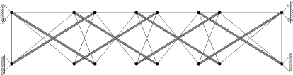
In this section, the planar Tensegrity beam arrangement to be used was based upon the model utilized in van de Wijdeven’s work. The model used in this application comprises of two modules, with pretension 30 cables and 8 struts, the ends of this beam are pined connected at the bottom and roller at the top (Figure 2).

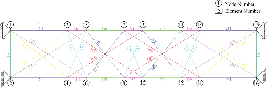
Figure 3 depicts the force density assumptions. Members shown in the same colors are thought to have equivalent force densities. The force density method, utilizing these intuitive assumptions, is then used to determine the initial coordinates and pretension forces in each member. The results are shown in Table 1.

Table 1 gives the summary of the force density and material properties of each member, and the stiffness and damping matrices can be formulated by these properties.

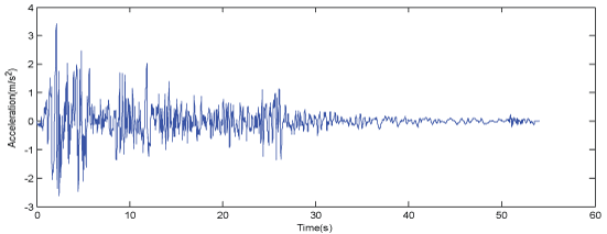
In order to observe the dynamic response and vibration control of the system under seismic excitation, the El Centro 1940 earthquake data is used as the excitation signal (Figure 4).

To optimize the control force on this system, the linear quadratic regulator algorithm will be used here. As is discussed above, this requires specifying weighting matrices, Q and R, which are defined as the following form:

$$Q=\begin{array}{l}\alpha \cdot \left[\begin{array}{l}{K}_b{O}_n\\ O_{n}M\end{array}\right]\\ R=\beta .I_n\end{array}\}(39)$$

Where α and β are the coefficients for weighting matrices determined by the designer.

In order to view the results of placing more weight on controlling the deflecting or minimizing the control force, three different sets of coefficients α and β will be considered:

$$\begin{array}{l}{Q}_1/R_1\alpha =2.5,\beta =0.1\\ Q_2/R_2\alpha =25,\beta =0.1\\ Q_3/R_3\alpha =25,\beta =0.01\end{array}\}(40)$$

Here, the LQR function in MATLAB will be used to evaluate the optimal gain. This function, gives the A and B parameters of the state space and specified weighting matrices,Q and R, gives the optimal gain V, namely:

$$V=lqr(A,B,Q,R)(41)$$

actuator force is then determined by the following equation:

$$F_i=V_i\cdot u(42)$$

Where u is the vector of displacements.

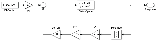
With the system and controller fully defined, the system, along with the control force, can be modeled in Simulink, the visual diagram of this system can be found in Figure 5.

As is shown in the above figure, the system is subjected to the seismic excitation which will be used at each degree of freedom. The excitation is evaluated in the state space and the displacements and velocities at each degree of freedom at time t are produced. These responses are then multiplied by the predetermined gain V of the controller, as well as the matrix which maps the gains to the appropriate nodes based on actuator placement. The additional force is added to the external excitation for the next step in the model. From this model, a plot of system response, actuator force, and member stress over the simulative time can be obtained.

Results and Discussion

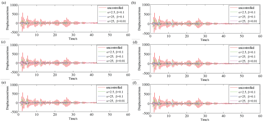
The above depicted simulation was conducted for all sceneries listed in the previous section, the El Centro 1940 earthquake data is used as the excitation signal and the response over a 60-second time interval was examined. Effects on displacement, maximum actuator force, internal forces in central members were all investigated.

The behavior of the response for each controller scenario was similar for each actuator placement, the plots of the responses of all scenarios can be found in Figures 6. Here, the red, blue, green, and magenta lines represent the uncontrolled response, Q₁/R₁ response, Q₂/R₂ response, and Q₃/R₃ response respectively. According to the definition of weighting matrices mentioned above, Q₂/R₂ the control parameters placed more weighting on minimizing controller output or mitigating deflections with respect to the Q₁/R₁ control parameters and Q₃/R₃ control parameters, respectively.

As can be seen, the uncontrolled responses have by far the largest maximum displacements. Take Figure 6 as an example, the maximum displacement of uncontrolled response is 569.69 mm at the time around 2.4 second, while the maximum displacement of controller scenario 1-3, is are 163.21 mm, 51.30 mm and 11.99 mm, respectively. The last two scenarios perform very similar and prove to nearly eliminate deflections of entirely in the system. The first scenario, whereas, still confirms to drastically reduce deflections with respect to the uncontrolled response. These results indicate that the LQR controller is more sensitive to increasing the importance of controlling the actuator force than with increasing importance on mitigating deflections, which means placing more weight on controlling the actuator force cause relatively larger increase in displacement while doing the opposite do not produce the same reduction in displacements.

The decision as to which control parameters would be best to utilize for the system depends on the system needs. If maintaining an identical shape is very important to the system, this can essentially be accomplished using the second control scenario or, if one wants to be conservative, the third scenario can be the best choice. If however, some deflections would prove to be acceptable in the system, a controller which maintains fairly small deflections can be accomplished using the first control scenario, which also proves to reduce the required input successfully.

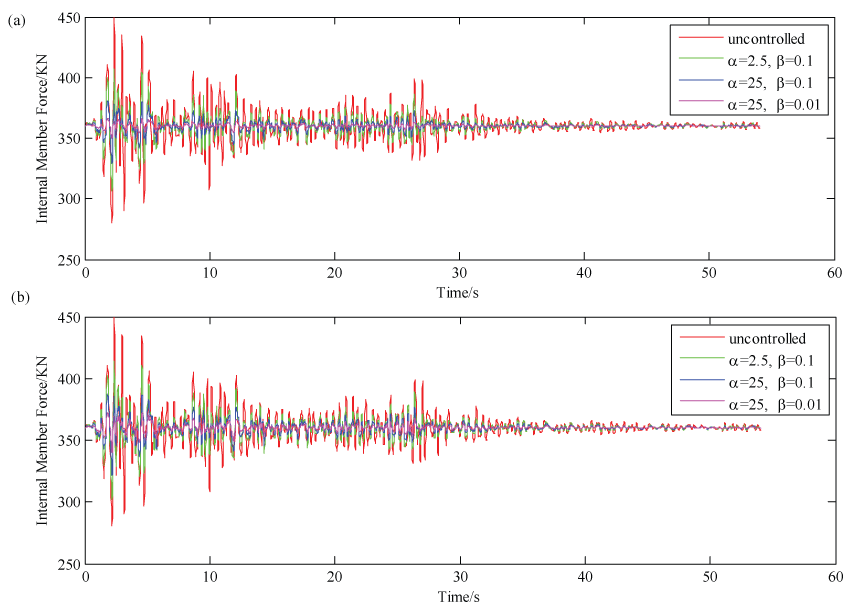
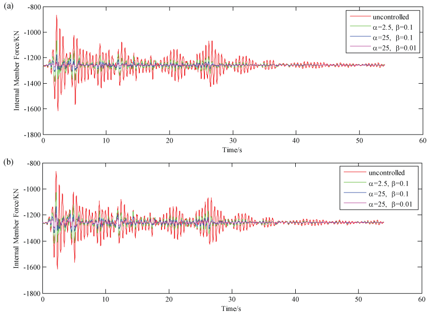
Meanwhile, the effect that the different controller scenarios on reducing internal member forces were also investigated in this paper. Considering the similarity of this pattern of behavior for all actuator placements, here, only two actuator placements were utilized. Also, cable 15 and strut 34 were chosen since they are central members and thus, more likely to be subjected to large internal forces. Figure 7 and Figure 8 show the internal forces of cable 15 and strut 34 over the simulative time.

By taking a close look at these figures, the relationship between the mitigation of deflection and the member stresses can be obtained directly. Just as in the case of deflections, the third controller almost entirely eliminated stresses in member, while, the second controller also successfully reduced member stresses. However, the first controller which placed less importance on weighting on minimizing controller output with respect to the second one still produced member stresses which are considerably less than in the uncontrolled scenario. It should be pointed out that in all controller scenarios, the cables remain to be always in tension and the struts remain to be always in compression, which are what should be expected. In other words, none of the components of the planar Tensegrity model with the properties given in Table 1 will be laid off due to the tension in struts or slackening of cables.

Moreover, all control scenarios demonstrated to minimize the variations and thus, maximum internal force in members. This means that when control is used, members can be made more slender as they will be less stressed. In the case of much control, particularity in the third control, members will essentially only need to be designed for their initial prestress forces.

Conclusion

Tensegrity systems are prestressed, self-supported configurations composing of tensioned cables and compressed struts. Due to their characteristics, they can be easily manipulated and moved to take on different shapes. This proficiency makes them great candidates to be incorporated into the idea of adaptable structures. This paper presents a theoretical analysis of dynamic response and vibration control of a Tensegrity structure subjected to seismic excitation using active control techniques. The control strategy adopted in this Tensegrity system is capable of meeting vibration control objective. Numerical results confirmed that LQR algorithm is possible to successfully actively control Tensegrity systems in order to minimize deflections, maintain shape, and ensure that the structures shape is always most optimal for the current loading. However, it does have a few limitations, for instance, the LQR controller utilizes a full state feedback which means the displacement and velocity at every node is given, while, this is not realistic in real structure. Apart from this, the issue of nonlinearity is not taken into account in this paper considering the simplification of the programming. Additionally, as a natural extension of this research, a linear observer (KF for instance) in conjunction with LQR control algorithm, known as LQG control formulation, might be employed to implement active control of Tensegrity structures.

References

1. Fuller RB (1962) Tensile-integrity structures. US Patent 3,063,521 A.
2. Snelson K (1965) Continuous tension, discontinuous compression structures. US Patent 3,169,611.
3. Motro R (2003) Tensegrity: Structural Systems for the Future. (1st edn), Kogan Page Science, London.
4. Motro R, Najari S, Jouanna P (1986) Static and Dynamic Analysis of Tensegrity Systems. In: Proceeding of the ASCE International Symposium on Shells and Spatial Structure. Computational Aspects Lecture Note in Engineering 26: 270-279.
5. Ben Kahla N, Moussa B, Pons JC (2000) Nonlinear dynamic analysis of tensegrity systems. Journal of the International Association for Shell and Spatial Structures 41: 49-58.
6. Oppenheim IJ, Williams WO (2001) Vibration and damping in three-bar tensegrity structure. Journal of Aerospace Engineering 14: 85-91.
7. Oppenheim IJ, Williams WO (2001) Vibration of an elastic tensegrity structure. European Journal of Mechanics A Solids 20: 1023-1031.
8. Sultan C, Corless M, Skelton RE (2002) Linear dynamics of tensegrity structures. Engineering Structures 24: 671-685.
9. Masic M, Skelton RE (2006) Selection of prestress for optimal dynamic/control performance of tensegrity structures. International Journal of Solids and Structures 43: 2110-2125.
10. Tan GEB, Pellegrino S (2008) Nonlinear vibration of cable-stiffened pantographic deployable structures. Journal of Sound and Vibration 314: 783-802.
11. Skelton RE, Helton JW, Adhikari R, et al. (2000) An introduction to the mechanics of tensegrity structures. Handbook on mechanical systems design, CRC, Boca Raton.
12. Djouadi S, Motro R, Pons JC, et al. (1998) Active control of tensegrity systems. Journal of Aerospace Engineering 11: 37-44.
13. Sultan C (1999) Modeling, design and control of tensegrity structures with applications. PhD thesis, Purdue Univ, West Lafayette.
14. Kanchanasaratool N, Williamson D (2002) Motion control of a Tnesegrity Platform. Communication in Information and System 2: 299-324.
15. Van de Wijdeven J, de Jager B (2005) Shape change of tensegrity structures: design and control. American Control Conference 2522-2527.
16. Bel Hadj Ali N, Smith IFC (2010) Dynamic behavior and vibration control of a tensegrity structure. International Journal of Solids and Structures 47: 1285-1296.
17. Nelson KE (2011) Active Control of Tensegrity Structures and Its Applications Using Linear Quadratic Regulator Algorithms. Massachusetts Institute of Technology, USA.
18. Crawley EF, Louis J (1989) Use of Piezoelectric Actuators as Elements of Intelligent Structures. AIAA Journal 25: 1373-1385.
19. Kalaycioglu S, Misra AK (1991) Approximate Solutions for Vibrations of Deploying Appendages. Journal of Guidance, Control, and Dynamics 14: 287-293.
20. Suleman A, Costa AP, Crawford C, Sedaghati R (1998) Wind Tunnel Aeroelastic Response of Piezoelectric and Aileron Controlled 3-D Wing. CanSmart Workshop Smart Materials and Structures, Proceedings.
21. Kobori T (1996) Future Direction on Research and Development of Seismic-Response-Controlled Structures. 11: 297-304.
22. Raja MG, Narayanan S (2007) Active control of tensegrity structures under random excitation. Smart Materials and Structures 16: 809-817.
23. Chen Y, Zhang WL, Gao HJ (2010) Finite frequency H∞ control for building under earthquake excitation. Mechatronics 20: 128-142.
24. Raja MG, Narayanan S (2009) Simultaneous Optimization of Structure and Control of Smart Tensegrity Structures. Journal of Intelligent Material Systems and Structures 20: 109-117.
25. Kebiche K, Kazi-Aoual MN, Motro R (1999) Geometrical non-linear analysis of tensegrity systems. Engineering Structure 2: 864-876.
26. Connor JJ (2003) Dynamic Control Algorithms: Time-Invariant Linear Systems. In: Connor JJ, Introduction to Structural Motion Control. Upper Saddle River, New Jersey, 458-664.