Modeling Distribution of Potassium in the Soil in Under Drip Irrigation

Abstract

In recent years, use of drip irrigation has been increased for many products, in a wide range of soil textures and structures. So far, any model has not been provided for distribution of potassium in the soil during irrigation. The purpose of this, research is modeling distribution of potassium in the soil, under drip irrigation. In this study, a physical model with dimensions 2.1 m × 0.9 m × 0.9 m was used to simulate a drip irrigation on the farm. The model was a transparent compartment of Plexiglas, where was divided into three distinct parts to provide carrying out three simultaneous testing. In each part of the compartment, a particular type of soil was tested. Both pulsed and continuous drip irrigation method was used. Two treatments, wastewater and irrigation water were used. By use of theorem of Buckingham and dimensional analysis, the model of potassium distribution in the soil was obtained. The model includes a number of equations which are able to estimate the amount of potassium in the soil. The results of the evaluation of the presented equations showed that the correlation coefficients between the measured and simulated values in clay soil and for the pulse and continuous drip irrigation systems were 0.929 and 0.941, respectively, for loamy soil, 0.959 and 0.935, respectively, and 0.929 and 0.909 for sandy soil, respectively. Estimated values with measured values were evaluated using the statistical indicators that confirmed the accuracy of the model. Therefore the model can be used for fertigation management in the continuous and pulsed drip irrigation method.

Keywords

Potassium, Pulse, Irrigation, Model, Soil

Notation

θ₀: Initial moisture; K (x, y): Potassium distribution in soil (mgL^-1); K₀: Initial potassium in soil (mgL^-1); G: Potassium concentration in irrigation water; q: Discharge flow from emitter (L^-T); K_s: Hydraulic conductivity in soil under saturation; R: radius of wetted soil (cm); V: Water applied (L); P_i: Predicted values; O_i: measured values; Ō: average of the measured values; RMSE: Root Mean Square Error; CRM: Coefficient Of Residual Mass; MAE: Mean Absolute Error; ME: Mean Error; R²: Coefficient of determination; n: The number of sample measurement

Introduction

In recent years the use of drip irrigation has been increased for many products and in a wide range of soil textures and structures. Numerous researches have been carried out to study the distribution of moisture and salts in the soil in drip irrigation. Potassium is one of the essential nutrients of the plant. It is important to know the concentration of potassium ions in the environment around the plant root in the soil. Classmen, et al. [1] proposed a mathematical model to simulate the absorption of potassium from the soil by plants. The simulation was based on ion transfer from the soil to the plant roots by mass flow and absorption of nutrients from the soil solution by plant roots. Ben Gal and Dudley [2] evaluated the fertigation of phosphorus in continuous and pulsed irrigation; they evaluated and simulated the distribution of water and phosphorus in Lysimetric in conditions of greenhouses. Before start of test, accumulation of phosphorus in different parts of model was measured. Comparison of the measured and simulated values by hydrous model showed that in under continuous irrigation with low rates in soil without plant, large phosphorus in the soil was available. Chen, et al. [3] studied the distribution of water and nitrate in the layered soil. In that study, three layered soils and two uniform soils were used. Also, the flow rate between 0.7-3.8 L/h was used. The results showed that the distribution of wetting front and nitrate depended on thickness of layers of soil and the flow rate of water in the soil. They observed nitrate accumulation at the boundary between the layers. Elemi, et al. [4] studied in soil columns in the laboratory using Hydrus-1D model to estimate the vertical distribution of phosphorus and leaching. The results showed that 98% of the total phosphorus concentration in soil column was 2.0 meters from the surface and gradually decline with increasing soil depth. The results showed that the phosphorus adsorption model was more than estimated values. Also, there was no good estimation model for the distribution of phosphorus in the soil when there was a preferential flow. "Honari, et al. [5]" in study of comparison of Hydrus-3D soil moisture simulation of subsurface drip Irrigation with experimental observations ,were showed the model have been placed in the excellent category for simulation of the soil water content.Soil moisture, salinity and nitrate concentration were measured weekly and compared with the obtained values by the developed model. The results showed that the mean absolute error (MAE) between measured and simulated values for moisture content was between 0.01 and 0.04, salinity at different depths between 0.02 and 0.04 and for distribution of nitrate between 1.0 and 1.97.

Several studies have been conducted in the field of water distribution in soil under drip irrigation using dimensional analysis which determines the depth and width of wetted soil [6-8]. Karimi, et al. [9] evaluated redistribution of wetting front in soil under subsurface drip irrigation. The results showed significant moisture content in soil at the redistribution stage. Considering the redistribution of moisture, the depth of irrigation water should be thinned down (less than before).

The model HYDRUS-2D simulates values of water content obtained at different lateral distances from a dripper at different soil depths at different times. The model closely predicts water content distribution at all distances, times and soil depths "Phogat, et al. [10]" Pulsed irrigation can slightly reduce water losses through the root zone when compared to continuous irrigation "Omkar, et al. [11]".

Although the Hydrous model is accurate and high-end, it requires a lot of input parameters, which are expensive and difficult to measure. The purpose of this research is to develop a model using dimensional analysis to estimate the distribution of potassium under continuous and pulse drip irrigation system in different types of soils. So far, the equations for the distribution of salts in the soil during irrigation are not provided. The development of the recent model allows us to estimate the concentration of potassium ions around the plant root.The objective of this study is providing general relationship for the distribution of potassium in the soil in pulsed and continuous drip irrigation system.

Material and Methods

In engineering, applied mathematics, and physics, the Buckingham π theorem is a key theorem in dimensional analysis. This theorem states that if there are n dimensional variables, they may be homogeneous equation, described by m fundamental dimensions; they may be grouped in n-m dimensionless groups.

The geometry of wetted soil together with distribution of minerals in the soil at the end of irrigation water depends on irrigation time, the volume of water applied, soil hydraulic conductivity, discharge of emitters, initial potassium of soil, soil moisture content and so on.

By using Buckingham theorem:

$$f\left(K,\theta ,G,q,K_s,V,t,R,{\theta }_0,K_0\right)\text{ = 0 (1)}$$

$$R\text{ = }\sqrt{D^2\text{ + }{Z}^2}\text{ (2)}$$

where K, θ, F, q, K_s, V, t, R, θ0, K₀ are initial potassium of soil, initial soil moisture content, the radius of the wetted soil, irrigation time, the volume of water applied, soil hydraulic conductivity, discharge of emitters, potassium concentration in irrigation water, soil moisture and soil potassium content.

Thus, in the problem, n = 10 and m = 3 (M, L and T) and n-m = 7, which it can be written as:

$$\left({\pi }_1,{\pi }_2,{\pi }_3,{\pi }_4,{\pi }_5,{\pi }_6,{\pi }_7\right)\text{ = 0 (3)}$$

The problem now is to find the π and s by arranging the ten parameters in to seven dimensionless groups as follows:

$${\pi }_1\text{ = }{q}^{a_1}{K}_s^{b_1}{G}^{c_1}V\text{ = }{\left(L^3{T}^{-1}\right)}^{a_1}.{\left(L{T}^{-1}\right)}^{b_1}.{\left(M{L}^{-3}\right)}^{c_1}{L}^3\text{ = }\left\{\begin{array}{c}{a}_1\text{= -}\frac{3}{2}\\ b_1\text{ = }\frac{3}{2}\\ c_1\text{ = 0}\end{array}\right.\text{ (4)}$$

$${\pi }_2\text{ = }{q}^{a_2}{K}_s^{b_2}{G}^{c_2}R\text{ = }{\left(L^3{T}^{-1}\right)}^{a_2}.{\left(L{T}^{-1}\right)}^{b_2}.{\left(M{L}^{-3}\right)}^{c_2}{L}^1\text{ = }\left\{\begin{array}{c}{a}_1\text{= -}\frac{1}{2}\\ b_1\text{ = }\frac{1}{2}\\ c_1\text{ = 0}\end{array}\right.\text{ (5)}$$

$${\pi }_3\text{ = }{q}^{a_3}{K}_s^{b_3}{G}^{c_3}K\text{ = }{\left(L^3{T}^{-1}\right)}^{a_3}.{\left(L{T}^{-1}\right)}^{b_3}.{\left(M{L}^{-3}\right)}^{c_3}.M{L}^{-3}\text{ = }\left\{\begin{array}{c}{a}_1\text{= }0\\ b_1\text{ = 0}\\ c_1\text{ = -1}\end{array}\right.\text{ (6)}$$

$${\pi }_4\text{ = }{q}^{a_4}{K}_s^{b_4}{G}^{c_4}\theta \text{ = }{\left(L^3{T}^{-1}\right)}^{a_4}.{\left(L{T}^{-1}\right)}^{b_4}.{\left(M{L}^{-3}\right)}^{c_4}\text{ = }\left\{\begin{array}{c}{a}_1\text{= }0\\ b_1\text{ = 0}\\ c_1\text{ = 0}\end{array}\right.\text{ (7)}$$

$${\pi }_5\text{ = }{q}^{a_5}{K}_s^{b_5}{G}^{c_5}t\text{ = }{\left(L^3{T}^{-1}\right)}^{a_5}.{\left(L{T}^{-1}\right)}^{b_5}.{\left(M{L}^{-3}\right)}^{c_5}\text{.}{T}^1\text{ = }\left\{\begin{array}{c}{a}_1\text{= }0\\ b_1\text{ = 0}\\ c_1\text{ = 0}\end{array}\right.\text{ (8)}$$

$${\pi }_6\text{ = }{q}^{a_6}{K}_s^{b_6}{G}^{c_6}{K}_0\text{ = }{\left(L^3{T}^{-1}\right)}^{a_6}.{\left(L{T}^{-1}\right)}^{b_6}.{\left(M{L}^{-3}\right)}^{c_6}\text{.}M{L}^{-3}\text{ = }\left\{\begin{array}{c}{a}_1\text{= }0\\ b_1\text{ = 0}\\ c_1\text{ = -1}\end{array}\right.\text{ (9)}$$

$${\pi }_7\text{ = }{q}^{a_7}{K}_s^{b_7}{G}^{c_7}\theta \text{ = }{\left(L^3{T}^{-1}\right)}^{a_7}.{\left(L{T}^{-1}\right)}^{b7}.{\left(M{L}^{-3}\right)}^{c_7}\text{ = }\left\{\begin{array}{c}{a}_1\text{= }0\\ b_1\text{ = 0}\\ c_1\text{ = 0}\end{array}\right.\text{ (10)}$$

In the above equations, flow rate (q), hydraulic conductivity (K) and potassium concentration in irrigation water (G) as repeating variables, potassium and the volume of water were applied, watering time, the radius of the water movement in the soil, soil moisture and raw potassium-were considered as non-recurring factors.

After solving the equations, to determine the coefficients a₁ to a₇ and b₁ to b₇ exponents of equations, π₁ to π₇ would be determined as follow:

$${\pi }_1\text{ = }{\left(\frac{K_s}{q}\right)}^{\frac{3}{2}}.V\text{ (11)}$$

$${\pi }_2\text{ = }{\left(\frac{K_s}{q}\right)}^{\frac{3}{2}}.R\text{ (12)}$$

$${\pi }_3\text{ = }\frac{K}{G}\text{ (13)}$$

$${\pi }_4\text{ = }\theta \text{ (14)}$$

$${\pi }_5\text{ = }\frac{K_s^{\frac{3}{2}}}{q^{\frac{1}{2}}}.t\text{ (15)}$$

$${\pi }_6\text{ = }\frac{K_0}{G}\text{ (16)}$$

$${\pi }_7\text{ = }{\theta }_o\text{ (17)}$$

π₁ to π₇ are dimensionless numbers and functions of K, θ, V, t, R, θ₀, K₀ with stars of their index variables have been shown. So, the equations would change as follow:

$$V^{*}\text{ = }{\left(\frac{K_s}{q}\right)}^{\frac{3}{2}}.V\text{ (18)}$$

$$R^{*}\text{ = }{\left(\frac{K_s}{q}\right)}^{\frac{1}{2}}.R\text{ (19)}$$

$$K^{*}\text{ = }\frac{K}{G}\text{ (20)}$$

$${\theta }^{*}\text{ = }\theta \text{ (21)}$$

$$t^{*}\text{ = }\frac{K_s^{\frac{3}{2}}}{q^{\frac{1}{2}}}.t\text{ (22)}$$

$$K_0^{*}\text{ = }\frac{K_0}{G}\text{ (23)}$$

$${\theta }_0^{*}\text{ = }{\theta }_o\text{ (24)}$$

The given non-dimensional numbers have the ability to multiply and divide, then the K* and V* functions are represented as a combination of several non-dimensional numbers π, which is as follow:

$$K^{*}\text{ = }{\pi }_3.{\pi }_7.\sqrt{{\pi }_6}\to K^{*}\text{ = }\frac{K{\theta }_0}{G}\sqrt{\frac{K_0}{G}}\to K\text{ = }\frac{K^{*}{G}^{1.5}}{{\theta }_o.K_0^{0.5}}\text{ (25)}$$

$$V^{*}\text{ = }\sqrt{{\pi }_1^2.{\pi }_2}\to {\left(\frac{K_s}{q}\right)}^{\frac{7}{4}}.R^{0.5}\text{ (26)}$$

By establishing relationships between dimensionless parameters, coefficients of these functions would be determined as follow:

$$K^{*}\text{ = }F\left(V^{*}\right)K^{*}\text{ = }{m}_1.V^{*n_1}\text{ (27)}$$

That in the above equation m1, m2 and n1, n2 are the constant values.

To return to the dimensionless parameter its dimensions, instead of V* and K*, the values should be replaced. The equations would be as follow:

$$K^{*}\text{ = }{m}_1.V^{*n_1}\to \frac{K{\theta }_o}{G}\sqrt{\frac{K_0}{G}}\text{ = }{m}_1\left({\left(\frac{K_s}{q}\right)}^{\frac{7}{4}}.R^{0.5}.V\right)\to K\text{ = }{m}_1.\frac{G^{1.5}}{{\theta }_o{K}_0^{0.5}}.{\left(\frac{K_s}{q}\right)}^{\frac{7}{4}{n}_1}.R^{0.5n_1}.V^{n_1}\text{ (28)}$$

Given the high ratios and power fit between non-dimensional numbers, the coefficients of the equations non- dimensions m1 and n1 were calculated.

These calculations were performed for all three types of soil texture for pulsed and continuous drip irrigation systems.

Statistical indicators to assess

To determine the accuracy of the model, it is required that the model be evaluated.

For this reason, Root Mean Square Error (RMSE), mean absolute error (MAE), mean error (ME), coefficient of residual mass (CRM) and coefficient of determination (R²) were used. Definitions of the statistical indicators are:

$$RMSE\text{ = }\sqrt{\frac{{\displaystyle {\sum }_{i\text{ = 1}}^n{\left(P_i-O_i\right)}^2}}{n}}\text{ (29)}$$

$$MAE\text{ = }\frac{1}{n}{\displaystyle {\sum }_{i\text{ = 1}}^n\left|P_i-O_i\right|}\text{ (30)}$$

$$ME\text{ = }\frac{1}{n}{\displaystyle {\sum }_{i\text{ = 1}}^n\left(P_i-O_i\right)}\text{ (31)}$$

$$CRM\text{ = }\frac{{\displaystyle {\sum }_{i\text{ = 1}}^n{O}_i-{\displaystyle {\sum }_{i\text{ = 1}}^n{P}_i}}}{{\displaystyle {\sum }_{i\text{ = 1}}^n{O}_i}}\text{ (32)}$$

$$R^2\text{ = }1-\frac{{\displaystyle {\sum }_{i\text{ = 1}}^n{\left(P_i-O_i\right)}^2}}{{\displaystyle {\sum }_{i\text{ = 1}}^n{\left(O_i-\overline{O}\right)}^2}}\text{ (33)}$$

Where P_i is predicted value, O_i measured, Ō is average value of the measured parameters and n is the number of sample measurement. RMSE represents the difference between the measured and predicted by the model .The closer to zero indicates that the model is more predictable less error. CRM overestimated or underestimated the model describes that if the value is negative indicator is underestimated and if positive value represents more than forecast model. R2 values show scattering between measured and predicted data by the model.

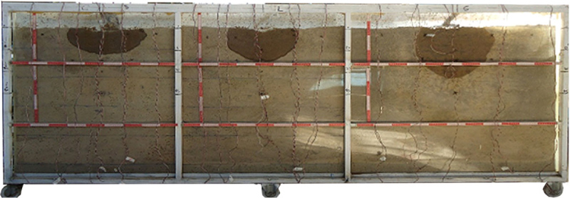
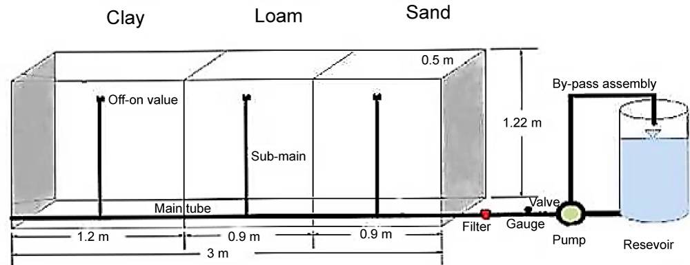
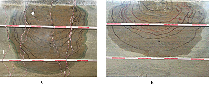
Test method: The tests were designed partly to the actual conditions on the farm with a drip irrigation system for simulation. In this study, a physical model with dimensions of 1.2 m × 0.9 m × 0.9 m was made to simulate a drip irrigation on the farm. The model was one transparent compartment of Plexiglas. The model has been divided into the three distinct parts until there are possibility of providing simultaneous testing for the three soils (Figure 1). In each part of the compartment, just one type of soil was tested. Because the horizontal distribution of water is more heavy soils, the container with the maximum length (1.2 meters) was allocated to heavy textured soils, and for light and medium textured soils, each compartment with a length of 0.9 m was allocated. Adhesive was applied to the inner wall and sand was spread on a wall to create almost roughness to prevent preferential flow during tests [12]. Water from the tank (with volume of 250 L) by the pump through the pipes with a diameter of 50 mm to the laterals with 16 mm and is delivered to emitters (Figure 2). From dripper Netafim regulated flow rate of 2.4 L/h was used. Wastewater of Tehran city and irrigation water for tests was used. Both pulsed and continuous drip irrigation methods were used. The experiments were carried out for the three soil samples. The characteristics of soils can be seen in the Table 1. For both systems, duration of irrigation was equal. For pulsed irrigation, after every hour, one hour no irrigation or break was applied.

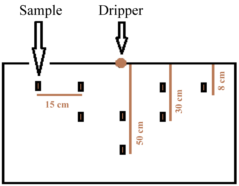
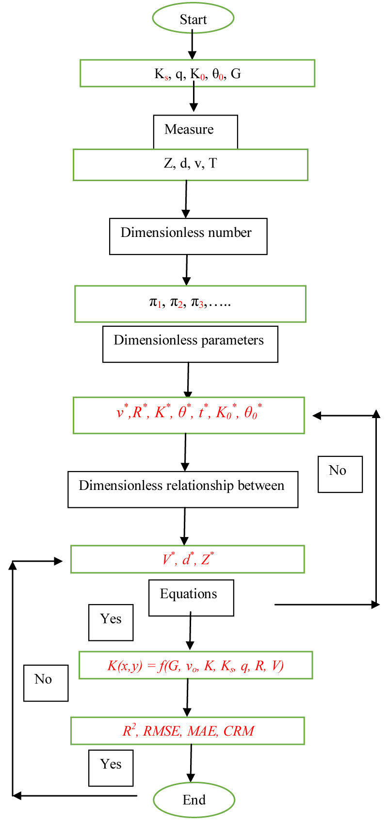
A Schematic of drawing of measurement points in the soil sample is shown in Figure 3. The characteristics of soils can be seen in the Table 1 and Table 2. For both systems, duration of irrigation was equal. For pulsed irrigation, after every hour, one hour no irrigation or break was applied. In Figure 4 Process flow chart of research is shown.

In Figure 4 the difference between pulsed and continuous wetting front of drip irrigation is shown.

Results

Determination the coefficients of m1 and n1

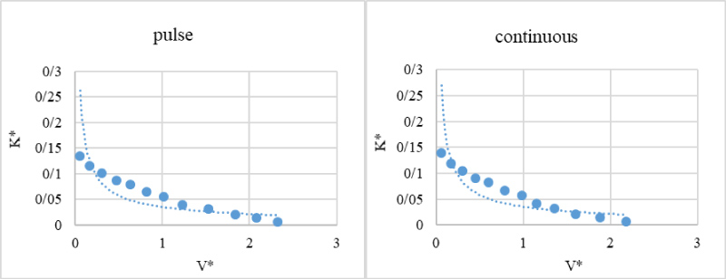
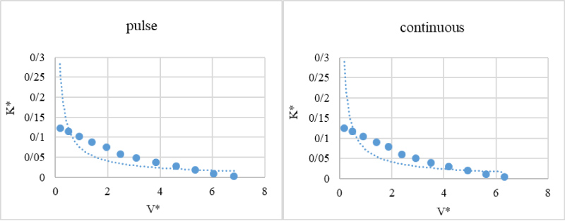
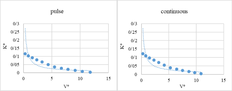
Determining the coefficients m1 and n1 in the sandy soil and clay loam soil for both pulsed and continuous irrigation were calculated. Dimensionless numbers K* and V* for number of tests were carried out from points of k and v curve were suitable fitted.

For three textures of soil clay, loam and sand under two irrigation method pulsed and continued irrigation suitable curve were fitted. In Figure 5 the difference between pulsed and continuous wetting front of drip irrigation is shown. According to Figure 6, Figure 7 and Figure 8 coefficients of n1 and m1 were determined. The coefficient of regression for all equations is well and suitable.

Distribution modeling of potassium in the soil by DAM

To obtain the modeling equations, at the first step, the coefficients of parametric equations were obtained. In the next step, the coefficient values in the relevant equations were replaced. The semi-empirical equations were obtained for estimating distribution of potassium in the soil around the roots surroundings. To determine the equation of distribution of potassium under pulsed drip irrigation in clay soil the coefficients obtained in the parametric equation were substituted in the formula for potassium distribution (Eq. 34).

Development of equations for distribution of potassium in the soil

Pulse Drip Irrigation (clay):

$$K^{*}\text{ = }{m}_1.V^{*n_1}\stackrel{\text{Replacement}}{\to }\frac{K{K}_0^{0.5}{\theta }_0}{G^{1.5}}\text{ = }{m}_1\left({\left(\frac{K_s}{q}\right)}^{\frac{7}{4}}.R^{0.5}.V\right)\stackrel{\text{Replacement}}{\to }K\text{ = }{m}_1.\frac{G^{1.5}}{{\theta }_o{K}_0^{0.5}}.{\left(\frac{K_s}{q}\right)}^{\frac{7}{4}{n}_1}.R^{0.5n_1}.V^{n_1}\stackrel{m_1\text{ = 0}\text{.0351 \& }{n}_1\text{ = -0}\text{.71}}{\to }K\left(x,y\right)\text{ = }0.0351\frac{G^{1.5}}{{\theta }_o{K}_0^{0.5}}.{\left(\frac{K_s}{q}\right)}^{-1.243}.R^{-0.355}.V^{-0.71}$$

And similarly for other textures the equations were developed, the final equations consist of:

Continuous Drip Irrigation (Clay): $K\left(x,y\right)\text{ = }0.0353\frac{G^{1.5}}{{\theta }_o.K_0^{0.5}}.{\left(\frac{K_s}{q}\right)}^{-1.26}.R^{-0.36}.V^{-0.72}\text{ (35)}$

Pulse Drip Irrigation (Loam): $K\left(x,y\right)\text{ = }0.071\frac{G^{1.5}}{{\theta }_o.K_0^{0.5}}.{\left(\frac{K_s}{q}\right)}^{-1.391}.R^{-0.396}.V^{-0.795}\text{ (36)}$

Continuous Drip Irrigation (Loam): $K\left(x,y\right)\text{ = }0.072\frac{G^{1.5}}{{\theta }_o.K_0^{0.5}}.{\left(\frac{K_s}{q}\right)}^{-1.4}.R^{-0.4}.V^{-0.8}\text{ (37)}$

Pulse Drip Irrigation (Sand): $K\left(x,y\right)\text{ = }0.0951\frac{G^{1.5}}{{\theta }_o.K_0^{0.5}}.{\left(\frac{K_s}{q}\right)}^{-1.475}.R^{-0.422}.V^{-0.843}\text{ (38)}$

Continuous Drip Irrigation (Sand): $K\left(x,y\right)\text{ = }0.0982\frac{G^{1.5}}{{\theta }_o.K_0^{0.5}}.{\left(\frac{K_s}{q}\right)}^{-1.4}.R^{-0.4}.V^{-0.8}\text{ (39)}$

where θ₀ is initial moisture, K(x,y) is Potassium distribution in soil (mg/L), K₀ is Initial potassium in soil (mg/L), G is Potassium concentration in irrigation water, q is Discharge flow from emitter (L/hr), K_s is Hydraulic conductivity in soil under saturation, R is radius of wetted soil (cm) and V is water applied (L). In this study, only discharge flow rate of 2.4 L/h was used to evaluate the potassium distribution equations in the soil.

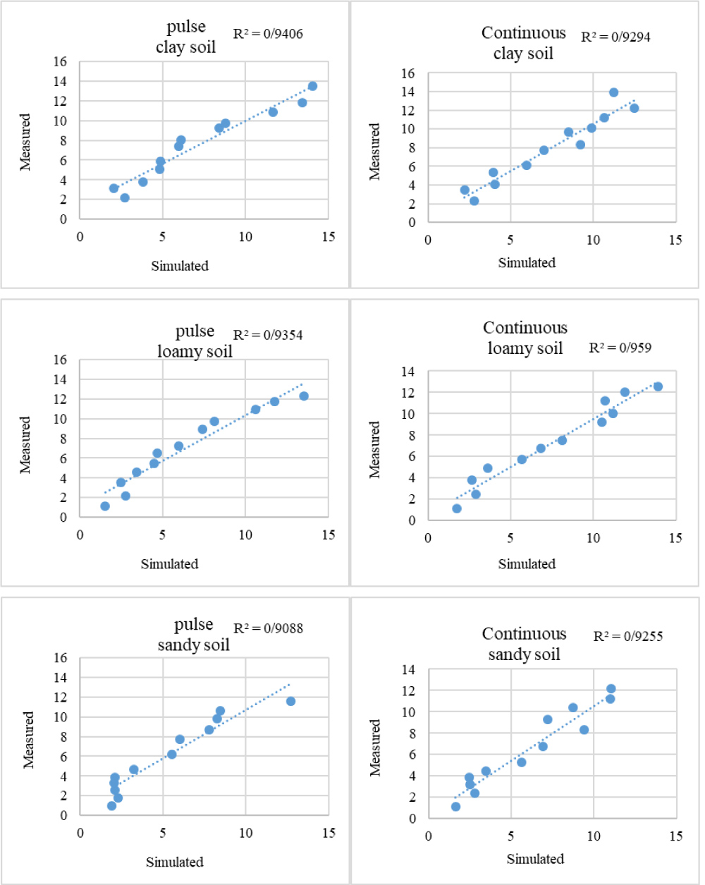
The results of the evaluation of the presented equations (Table 3) showed that the correlation coefficients between the measured and simulated values in clay soil and for the pulse and continuous drip irrigation systems were 0.929 and 0.941, respectively, for loamy soil, 0.959 and 0.935, respectively, and 0.929 and 0.909 for sandy soil, respectively (Figure 9). Finally, it can be concluded that the results of correlation coefficients indicated that the equations have a high efficiency for estimating the distribution of potassium in the soil.

The results of statistical parameters showed that statistical parameters were acceptable in these treatments, which indicates that the model has an acceptable performance in estimating the distribution of potassium in the soil.

Comparison similar studies and working conditions and the results with this study in shown in Table 4.

Conclusions

In this study, by dimensional analysis method to estimate concentration of salts in the soil under pulsed and continuous drip irrigation, a number of equations was extracted. In these equations, potassium concentration is a function of initial moisture content of soil, initial potassium of soil, hydraulic conductivity of soil and water volume in the soil and flow rate of dripper. The equations were derived for sandy, loamy and clay soils. The equations, with statistical indicators were evaluated. The results of the evaluation of the presented equations showed that the correlation coefficients between the measured and simulated values in clay soil and for the pulse and continuous drip irrigation systems were 0.929 and 0.941, respectively, for loamy soil, 0.959 and 0.935, respectively, and 0.929 and 0.909 for sandy soil, respectively. The results indicated that the proposed model is properly able to estimate the potassium concentration with high accuracy. The development of the recent model allows us to estimate the concentration of potassium ions around the plant root. Therefore, model can be used as a tool to manage irrigation fertilizer. This study have commercial significance and can be find application area such as in soil fertility and nutrient management.

Acknowledgment

We thank all who in one way or another contributed in the completion of this research. We give deep thanks to the Professors at the Irrigation and drainage engineering Department, workers of laboratory, and other Colleagues of the faculty of agriculture and natural resources in University of Tehran.

References

1. Claassen N, Syring KM, Jungk A (1986) Verification of a mathematical model simulating potassium uptake from soil. Plant and Soil 95: 209-220.
2. Ben Gal A, Dudley LM (2003) Phosphorus availability under continuous point source irrigation. Soil Science Society of American Journal 67: 1449-1456.
3. Chen JS, Mansell RS, NKedi Kizz AP, et al. (1996) Phosphorus transport during transient, unsaturated water flow in an acid sandy soil. Soil Science Society of American Journal 60: 42-48.
4. Elmi A, Nohra JSA, Madramootoo CA, et al. (2012) Estimating phosphorus leachability in reconstructured soil columns using Hydrus-1D model. Environmental Earth Sciences 65: 1751-1758.
5. M Honari, A Ashrafzadeh, M khaledian, et al. (2017) Comparison of Hydrus-3D soil moisture simulation of subsurface drip Irrigation with experimental observations in the south of France. Journal of Irrigation and Drainage Engineering 143.
6. Mirzaei F, Liaghat M, Sohrabi T, et al. (2006) Soil from linear source under drip tape-irrigation system. Journal of Agricultural Engineering Researches 6: 53-66.
7. Singh P, Sastry VRB, Garg AK, et al. (2006) Effect of long term feeding of expeller pressed and solvent extracted karanj (Pongamia pinnata) seed cake on the performance of lambs. Anim Feed Sci Technol 126: 157-167.
8. Rodríguez-Lázaro D, Lombard B, Smith H, et al. (2007) Trends in analytical methodology in food safety and quality: Monitoring microorganisms and genetically modifed organisms. Trends Food Sci Technol 18: 306-319.
9. Karimi B, Mirzaei F, Shorabi T (2013) Evaluation of redistribution of wetting front in soil under subsurface drip irrigation. Water and Soil Science 25: 141-152.
10. Vinod Phogat, Mahalakshmi Mahadevan Mark Skewes, James W Cox (2012) Modelling soil water and salt dynamics under pulsed and continuous surface drip irrigation of almond and implications of system design. Irrigation Science 30: 315-333.
11. Omkar D Gaonkar, G Suresh Kumar, Indumathi M Nambi (2016) Numerical investigations on pesticide fate and transport in an unsaturated porous medium for a coupled water and pesticide management. Environmental Earth Sciences 75: 1232-1232.
12. Kandeloos MM, Simune J (2010) Numerical of water movement in a subsurface drip irrigation system under field and laboratory conditions using hydrus-2D. Agricultural Water Management 97: 1070-1076.