Journal of Aerospace Engineering and Mechanics

Numerical and Experimental Study of Liquid Cryogenic Jet around a Space Plane and Its Ignition Risk

Abstract

Ariane Group is currently developing space vehicles using new LOx/LCH₄ propulsion technology. Venting or draining out methane from the tanks in flight at various altitudes concerns the safety management. This paper is focusing on the modeling of liquid methane draining around a moving space plane. A cryogenic round jet in an air crossflow has to be considered. However, the computational cost for a vaporizing liquid jet model is too high with respect to the goals of the study. A more time-friendly densified gas model has thus been developed. Experiments on liquid nitrogen were conducted to validate the numerical results. Numerical and experimental jet trajectories are in the same order of magnitude. Liquid column height is also properly modeled. The model is thus validated for pre-study calculations where global behaviors need to be determined without a prohibitive cost.

Keywords

Cryogenic jet, Densified gas model, Crossflow, Space plane, Methane

Nomenclature

Introduction

Methane possesses several advantages over other liquid rocket fuels such as hydrogen. For instance, its higher density reduces overall dimensions, and its higher liquefaction temperature leads to an easier implementation. Ariane Group is working on engines using liquid methane and liquid oxygen for various applications. One of these is a manned spaceplane, capable of take-off from an airport and to reach space to experience micro-gravity for several minutes. For safety management purpose, the risk of explosion near the vehicle for an emergency draining of the tanks is investigating. It might indeed be needed to evacuate the methane and oxygen from the tanks before landing if the rocket engine malfunctions. This emergency scenario should deal with a cryogenic jet in an air crossflow.

A gaseous jet in crossflow has been widely studied both experimentally [1-4] and numerically [5-7]. The injection of a gas perpendicularly to a flow creates a recirculation zone immediately behind the injected gas and modifies the primary flow trajectory. However, cryogenic jets in crossflow under low pressures and temperatures behave differently and have not been studied yet. The draining configuration is not encountered in the literature as a vast majority of the data regarding cryogenic liquid jets is given for engine conditions (coaxial injection, high pressures and temperatures). A literature review found that cryogenic jets in crossflow under standard pressures are also poorly documented. Richards [8] studied this type of flows experimentally but in a different configuration. The injection diameter is of only 0.5 mm and the air hotter (300-580 K), leading to a liquid/gas momentum flux ratio order of magnitude greater than in our study (Table 1). Thus, it is of great interest to study experimentally and numerically cryogenic jets under standard conditions. Moreover, numerical simulation of cryogenics is very demanding to accurately combine vaporization, liquid/gas interface and both liquid and gas flows. The present work reports the densified gas model and its comparison with experimental data. This model lowers the calculations time and cost by using an ideal gas law with adapted parameters, instead of modeling a diphasic flow. The theory and equations for the study are discussed in section 2. The comparison with experimental data is presented in section 3.1.3. Once the model is validated against experimental data, it is applied in the numerical calculation around the plane in section 4.

Theoretical Considerations

Liquid jets in crossflow

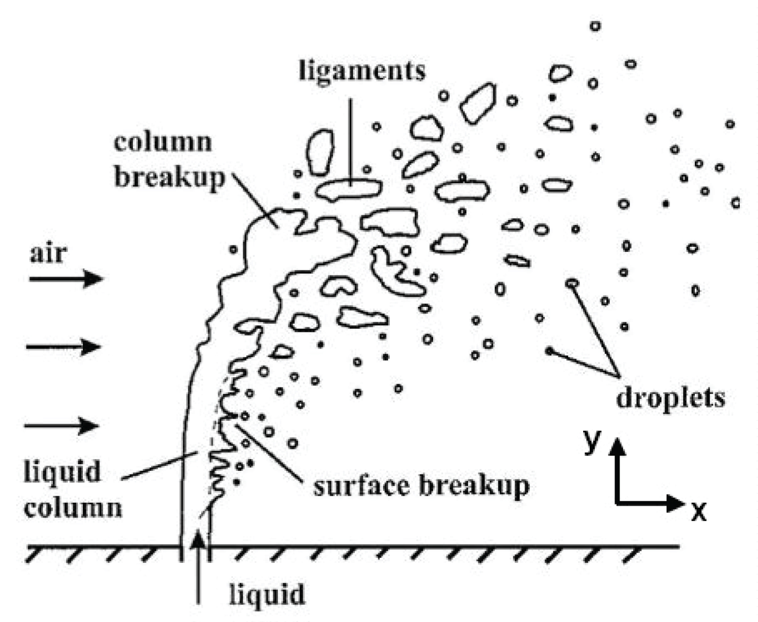
Methane is first assumed to come out in liquid state from the tanks without vaporizing. A cryogenic liquid usually differs from a standard liquid by both its pressure and its temperature. For a cryogenic jet at standard conditions, the vaporization rate is very important and is therefore a source of instability. Moreover, depending on the pressure and temperature differential between the tank and the atmosphere, flash evaporation can occur as determined by Witlox [9]. Because of cryogenic temperatures, an ice layer upward the injector is observed, which has an influence on the jet trajectory [8]. A non-evaporating liquid jet behaviour is presented in Figure 1 [10].

In this study, only subsonic speeds will be considered given the relatively low flight speed encountered by the plane in flight (Mach 0.4). Right after the injection, a liquid column is created perpendicularly to the wall. Farther away from the injector, this column is bended by the crossflow and fragments of liquid are sheared apart. At some point, the liquid column breaks into fragments, which will eventually break into droplets.

$$\mathrm{Re}i=\frac{\rho iuidjet}{\mu i}=\frac{inertialforce}{viscousforce}\left(1\right)$$

$$Wei=\frac{\rho i{u}_i^{2}djet}{\sigma }=\frac{inertialforce}{surfacetension}\left(2\right)$$

$$q=\frac{\rho l{u}_l^2}{\rho g{u}_g^2}=\frac{liquidmomentumflux}{gasmomentumflux}\left(3\right)$$

Several non-dimensional parameters are used to improve the comparison between different liquid jets. Three of them are presented in the Equations (1) to (3) where subscript i describes either the liquid phase l or the gaseous phase g. The trajectory of a fully developed liquid jet is essentially determined by the parameter q and the jet penetration is indeed growing with this parameter according to both our experiments and the ones by Richards.

Table 1 resumes the non-dimensional parameters for cryogenic nitrogen study which had been carried out by Richards [8] and the flight-related parameters for our Spaceplane study with liquefied methane. Despite the differences between all parameters, both studies should be using the same atomization breakup regime according to the classification of Faeth, et al. [11]. Our Ohnesorge number Oh lies into the 1.10^-4 - 1.10^-3 interval, well under the lower limit for stable jets and the gaseous Weber number Weg lies above the lower limit of the atomization regime. However, considering the major disparity between both studies, experimental correlations derived from the results of Richards are irrelevant in this work.

Flammability limits and auto-ignition

This study aims at defining the explosion risk when the Space Plane dumps rocket propellants in flight. It is therefore important to study flammability limits of methane, which represent the amount of fuel that allows inflammation. Under the Lower Flammable Limit (LFL), fuel is too diluted for ignition to occur. Above the Upper Flammable Limit (UFL), fuel is too concentrated for ignition to occur. From a safety management point of view, it is recommended to maintain methane concentration under the LFL at all times.

Methane is a relatively common gas whose flammability limits are well known for various pressures and temperatures. However, both atmospheric pressure and temperature are low in this study. Coward, et al. [12] illustrated the effect of decreasing pressure and temperature on flammability limits. The more pressure and temperature decrease, the narrower the flammability limits are. More recent papers focus on the flammability limits for low temperatures or low pressures [13-16]. At atmospheric pressure, these authors obtained substantial differences for the LFL at 150 K, respectively 6.3%, 6.64% and 5.45% in mole fraction. From a risk assessment point of view, these three results in the same conditions are not suitable. Expanding the correlations from Cui, et al. [13] to our operating pressure gives a LFL of 5.57% and an UFL of 14.07%. Common flammability limits of 5 and 15% are then used in this study due to these literature uncertainties.

Another important parameter is the auto-ignition temperature. Several gases such as methane can ignite under the influence of temperature. No external source is necessary. As for flammability limits, the ignition temperature is dependent on the type of device used to measure it. A common low temperature of auto-ignition for methane is 873 K according to Kundu, et al. [17]. This value will be used in this study.

Model Comparison with Experimental Data

Densified gas model

Physical model: Modeling of liquid jets is of great interest for several industries and is, thus, widely studied [18-23]. The scales involved and the type of model have a significant influence on the precision and duration of the calculation. In this study, the scales are important -several meters- and the use of a two-phase flow is not compatible with other prerequisites including the calculation time. A single law of state is used throughout the domain, the perfect gas law (Equation (4)). Perfect gas law was preferred over a real gas approach or more complete models such as the GERG-2008 [24] equation because precise flow or temperature fields are not needed in a pre-study phase. The industry can't afford to model two-phase flows accurately and has thus developed several means to compute such flows without the numerical burden they represent. One of the models developed is the HEM model, first proposed in 2014 [25]. While requiring less computational resources than 6 equations models and being more precise than other 4 equations mixture models, our software can't implement such a law through user defined subroutines.

In the real system, the pressure inside the methane tank is of 5 bar. Numerically, at the draining orifice, this tank pressure is artificially increased to 255 bar to obtain the density of a liquid in the perfect gas law. This artifice is used only locally to respect the draining mass flow rate of a liquid.

$$P=\rho \frac{R}{M_{mix}}T\left(4\right)$$

However, properties such as enthalpy, specific heat or thermal conductivity are gaseous ones and not liquid even at the draining orifice.

Considering the dangerousness of methane in wind tunnel tests, liquid nitrogen was preferred for the experiments. The following numerical calculations presented are thus for liquid nitrogen only. To mimic liquid nitrogen at a temperature of 75 K and a density of 816.7 kg/m³, the pressure must be raised to 180.6 bar in the Equation (4).

Equations: The calculations were executed through CFD-ACE, a multiphysics finite volumes software developed by ESI-GROUP [26]. For these simulations, turbulent flows with heat transfer and chemical diffusion are modeled. Equation (5) is used for each species n. Bold symbols represent vectors. The subscript i stands for inviscid terms whereas the subscript v stands for viscous terms.

$$U=\left(\begin{array}{l}\rho n\\ \rho nu\\ \rho nv\\ \rho nw\\ \rho nH+pn\end{array}\right),Fi=\left(\begin{array}{l}\rho nu-Jnx\\ \rho n{u}^2+pn\\ \rho nvu\\ \rho nwu\\ \rho nuH-keff\frac{\partial T}{\partial x}\end{array}\right),$$

$$Fv=\left(\begin{array}{l}0\\ \tau xx\\ \tau xy\\ \tau xz\\ u\tau xx+v\tau xy+w\tau xz\end{array}\right)$$

$$Gi=\left(\begin{array}{l}\rho nv-Jny\\ \rho nuv\\ \rho n{v}^2+pn\\ \rho nwv\\ \rho nvH-keff\frac{\partial T}{\partial y}\end{array}\right),Gv=\left(\begin{array}{l}0\\ \tau yx\\ \tau yy\\ \tau yz\\ u\tau yx+v\tau yy+w\tau yz\end{array}\right),$$

$$Hi=\left(\begin{array}{l}\rho nw-Jnz\\ \rho nuw\\ \rho nvw\\ \rho n{w}^2+pn\\ \rho nwH-keff\frac{\partial T}{\partial z}\end{array}\right)$$

$$Hv=\left(\begin{array}{l}0\\ \tau zx\\ \tau zy\\ \tau zz\\ u\tau zx+v\tau zy+w\tau zz\end{array}\right),S=\left(\begin{array}{l}0\\ 0\\ 0\\ 0\\ 0\end{array}\right)$$

$$\frac{\partial U}{\partial t}+\frac{\partial \left(Fi-Fv\right)}{\partial x}+\frac{\partial \left(Gi-Gv\right)}{\partial y}+\frac{\partial \left(Hi-Hv\right)}{\partial z}=S\left(5\right)$$

The species viscosity is modeled through the Sutherland's law (Equation (6)).

$$\mu =\frac{A{T}^{3/2}}{B+T}\left(6\right)$$

Both specific heat and thermal conductivity use a five-order polynomial in temperature, values obtained through the NIST database [27].

Finally, thermal, and chemical diffusion are modeled through Equation (7).

$$jn=-\rho nDn\nabla Yn-\rho n{D}_n^T\nabla \left(\ln T\right)\left(7\right)$$

Turbulence is solved with the SST k-ω model from Wilcox [28]. This RANS model is well suited for aerodynamic flows and cost effective. A standard wall function is used to limit ourselves to y+ values between 30 and 150 at the wall. The parameters k and ω are not directly specified, as the turbulence intensity I and the length scale c allow to find them and are more easily accessible.

$$I=\frac{u^{\prime }}{U}=\frac{\sqrt{\frac{2}{3}k}}{U}\left(8\right)$$

$$lc=C\mu \frac{k^{1/2}}{\omega }\left(9\right)$$

Solver: Pressure and velocity must be linked to solve the Navier-Stokes equations. The Semi-Implicit Method for Pressure Linked Equations-Consistent (SIMPLEC) [29] is used for this purpose. This iterative process, derived from the SIMPLE algorithm [30], is based on the same steps as SIMPLE except for the under relaxation of the pressure term p, which is not needed by the mean of different correction coefficients in the pressure correction. A comparison of the numerical results with experimental values is needed. Our experiments can only reproduce the parameter $q=\frac{{\rho }_{liq}{u}_{{}_{liq}}^2}{{\rho }_{gaz}{u}_{gaz}^2}$ whereas the Reynols number $\mathrm{Re}=\frac{\rho ud}{\mu }$ and the Weber number $We=\frac{\rho u^{2}d}{\sigma }$ will have different values (Table 2). However, the parameter q is the main driver of the jet trajectory according to the bibliography. The experiments should thus be able to reproduce the jet trajectory and be used as a comparison for the numerical model.

Experimental setup

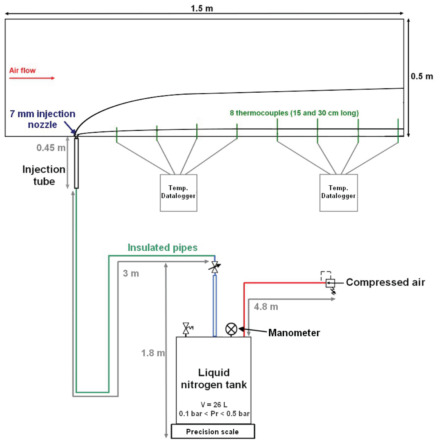
The wind tunnel is 1.5 m long for a square section of 50 cm wide. The air velocity can be varied to a degree of 0.1 m. s^-1. 8 J-type thermocouples of 1 mm in diameter, placed into the symmetry plane of the tunnel, are linked to data loggers. These thermocouples are located 10, 30, 40, 50, 60, 70, 80 and 110 cm away from the nitrogen injector. The data loggers have an acquisition frequency of 1 Hz and a precision of 0.7K. The overall precision on temperature, combining thermocouples and dataloggers, is of 2.9K as thermocouples for the range of temperatures involved have a precision of 1.2K. The experimental setup consists in a liquid nitrogen tank, pressurized between 0.1 and 0.4 barg. The drained mass flow rate is measured through a precision scale PCE-SD 30SST C placed under the tank. The scale records two mass values per second with a precision of 10 g (0.3% of the maximum mass). The nitrogen is transported to the wind tunnel with insulated pipes of 3 m long and 10 mm in diameter and injected through a PMMA injector with an inner diameter of 7 mm. As shown in Figure 2, nitrogen is introduced upward into the air flow from the bottom of the tunnel. Due to the experimental setup, misty flows are expected at the injection. However, these types of flows are also expected during the draining of methane in flight.

The reproducibility of the experiments and the influence of several parameters are explored with several configurations (Table 3). Trajectories and liquid column height are extracted from videos of the jet. Trajectories are measured with a precision of 2 cm. Liquid height is more precise, with an overall precision of 5 mm. Video quality is preferred over frames per second rate to facilitate the trajectory extraction. The widest videos are taken at 25 fps whereas the ones focused on the injector are at 60 fps.

Grid convergence

Several grids were tested for the wind tunnel configuration. The same geometry and the same type of grid were used. The main validation parameter was the temperature at the last thermocouple. The experimental temperature for the configuration studied is of 291.1 K. Table 4 contains three of the grids tested.

The third grid yields to the best temperature precision with a converged calculation. Under 9.0 × 10⁵ cells, the convergence is hard to achieve. Over 3.3 × 10⁶, the temperature precision is not better, and the calculation time rises. Grid number 3 will thus be used for our calculations.

Results

Outer trajectory: Pulsations are noticed on the jet mass flow rate. Additional measurements revealed two periodical pulsations, one at 33 Hz and another at 0.25 Hz. Several reasons might explain this behavior, such as small ice formation within the tank due to compressed air humidity, excessive heat transfer at pipes connections causing partial vaporization or cavitation. The jet pulsation makes the trajectories exploitation complex. An image in fact captures several mass flow rates at several locations. The Figure 3 presents an image taken from the video. Therefore, this work focuses only on initial tens centimeters of the jet to validate the trajectories.

The contrast is enhanced by a blue LED placed at the injector. The jet is clearly visible by the mean of water ice formed by the solidification of air humidity in contact with the cold jet. The numerical outer trajectory is obtained by a temperature condition of 273 K.

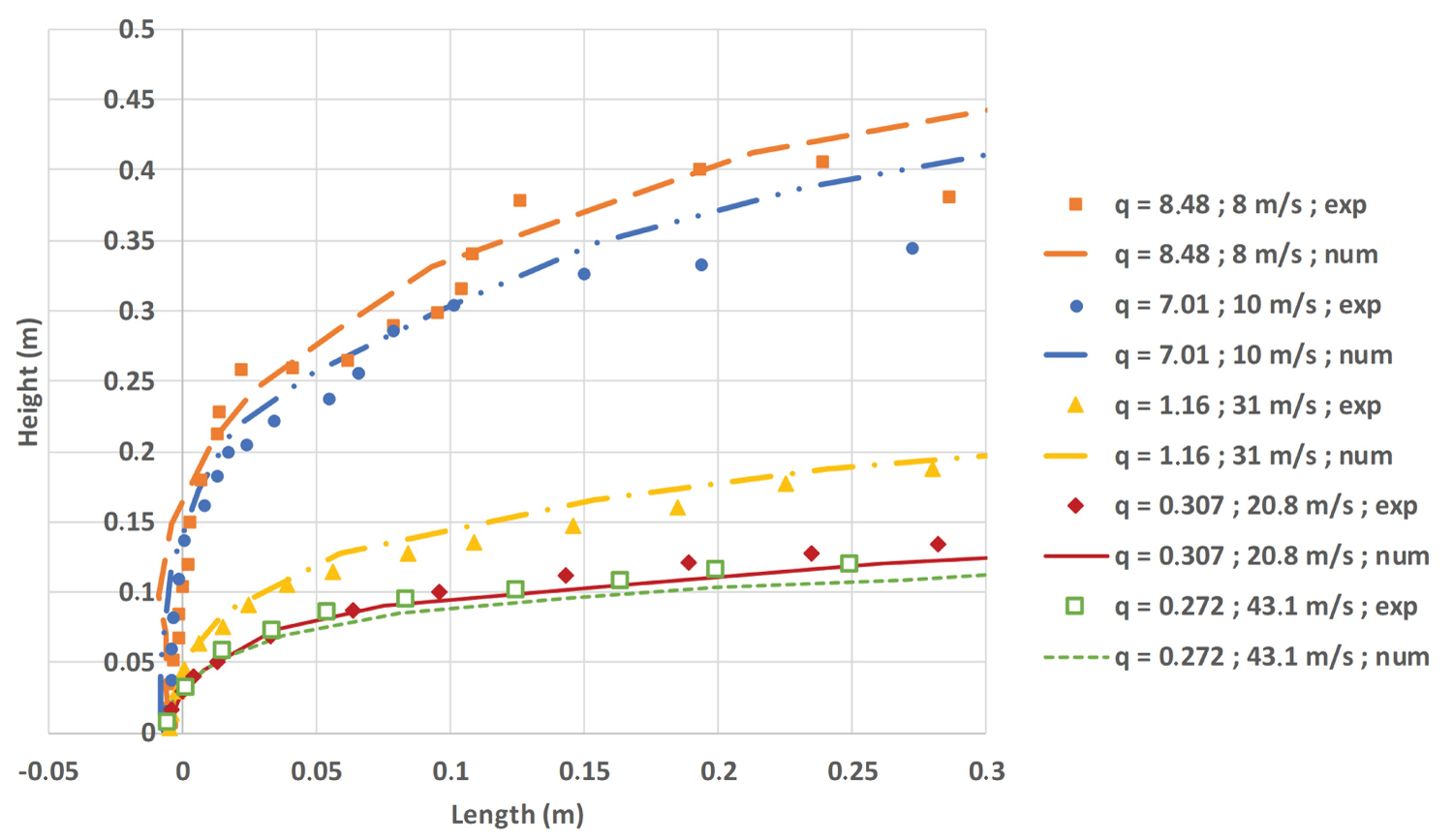
The results for a wide range of q parameter are exposed on Figure 4. The dots represent the experimental results whereas the lines represent the numerical ones.

A good agreement between experimental and numerical results is given by the Figure 4. The wind tunnel Reynolds number is more than doubled between the green pointed plot and the red solid plot (see Table 5) with small influence on the jet trajectory.

At the same time, the liquid Weber number drops from 478 to 126, with also no significant effect. These two behaviors highlight the predominance of the q parameter for the jet trajectory. At high q values, the jet is experiencing a modification of its trajectory after 0.1 m. This modification is due to the combination of jet instability and low wind speed values. Between 0.1 and 0.3 m, we are in fact observing the trajectory of a jet with a lower mass flow rate, due to the time needed to stabilize the jet between measurements. Some results at the end of the wind tunnel are not associated with the mass flow rate at the time of the image capture and thus are not representing the proper q number calculated with the mass flow rate.

Liquid column: The liquid column length is of prime importance to validate the numerical model. Numerically, the liquid cone length is estimated based on a temperature criteria. A temperature of 77 K is chosen, corresponding to the nitrogen boiling temperature under atmospheric pressure. The pressure change in the air flow due to both the singular and regular pressure loss and the air speed is only affecting slightly the ambient pressure (around 1500 P a of pressure loss). The temperature can thus be kept at 77 K. Experimental length is determined with the help of videos taken in the vicinity of the injector.

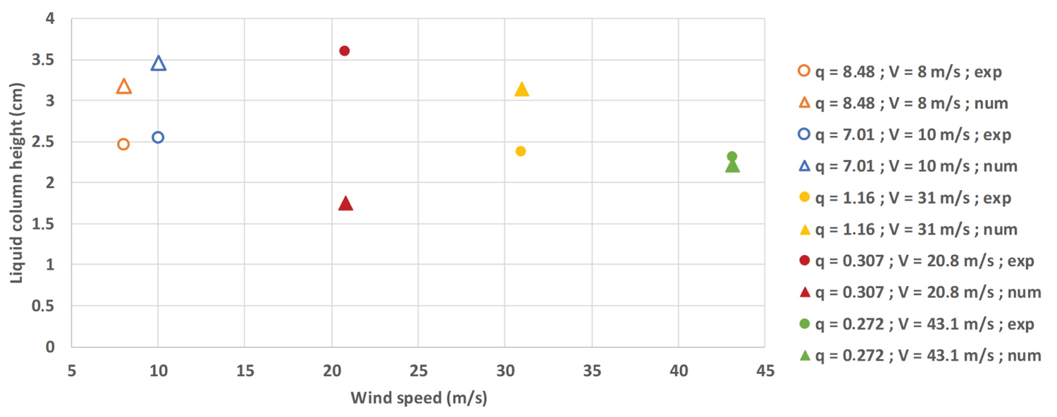
Once injected into the air flow, the liquid will rapidly vaporize due to its cryogenic nature, leading to a liquid column of only a few centimeters high (Figure 5). The dots represent the experimental values, the triangles the numerical ones. A large discrepancy is noticed between the experimental and numerical values for q = 0.307, which can be explained by the densified gas model principle. For q = 0.307, the nitrogen mass flow rate is of 13.8 g.s^-1, which is two to three times less than other mass flow rates used for this Figure. Numerically, when the mass flow rate is small, the gas will get warmer quicker than its liquid counterpart. The temperature difference between numerical and experimental results will decrease as the mass flow rate increases.

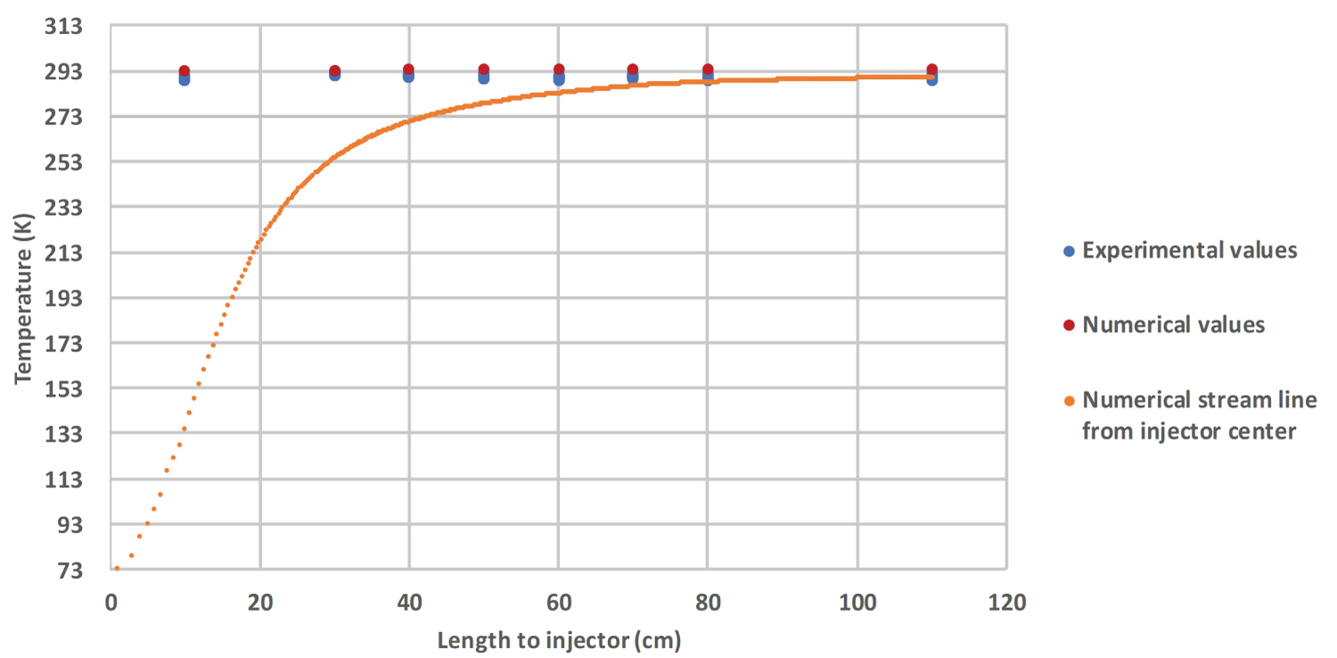
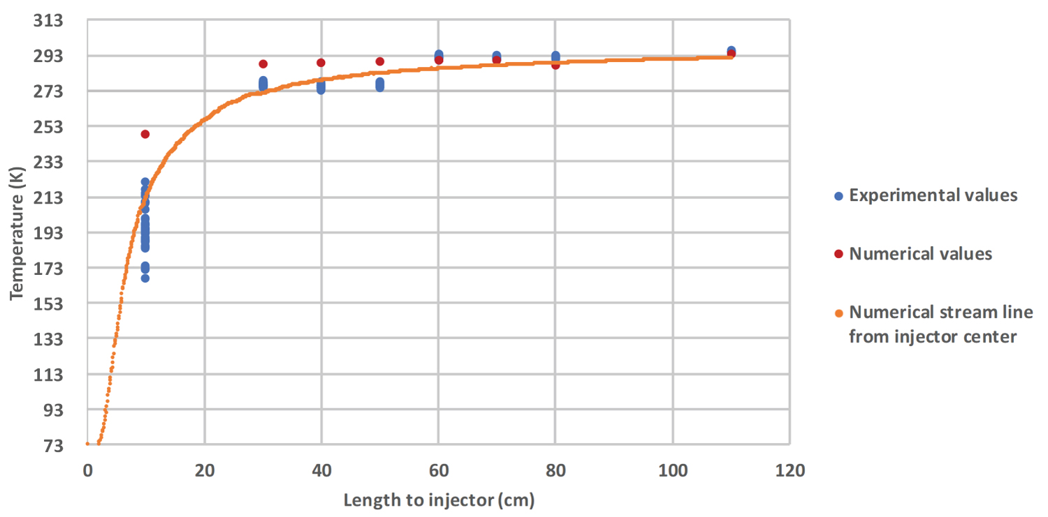
Temperature's profile: Numerical temperatures extracted from simulations are confronted with the readings of the 8 thermocouples. A streamline coming from the center of the injector is added on the Figure 6 and Figure 7, showing the trajectory of the core of the jet. When the thermocouple is placed outside of the liquid jet, numerical and experimental results are in relatively good agreement (Figure 6). As soon as the thermocouple lies within the jet (experimental values close to the streamline values), the difference between the experimental and the numerical temperatures increases (Figure 7). Globally, the numerical temperature is hotter than the experimental one, with a difference of 80 K close to the injector. This behavior might be explained by an easier mixing between the gases in the numerical simulation, due to the densified nature of nitrogen. One can observe a rapid increase in both numerical and experimental temperatures, with a rising from 75 K to 298 K in less than 1.1 m (horizontal length).

Conclusion

An experimental setup using liquid nitrogen was tested in a wind tunnel. The liquid nitrogen jet was injected vertically upward to simulate the injection of liquid cryogenic fuel in a perpendicular flow. The mass flow rate of the nitrogen and the wind tunnel speed were adjusted to mimic several flight configurations. The outer jet trajectory, the liquid column height and the temperatures profile were measured. Numerical simulations of the tests were undertaken. The densified gas model was satisfactorily confronted to experimental results. We will now apply this model to the draining of liquid methane from a moving space plane, where relevant experimental data are unavailable.

Numerical Calculations for the Space Plane Flight

Model parameters

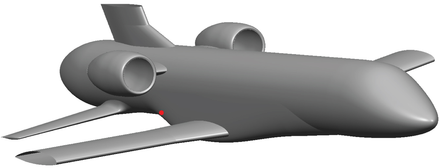
Draining procedure was simplified to occur at a constant altitude of 2 km. Using the US Standard Atmosphere [31], atmospheric temperature and pressure were determined at 275K and 0.795 bar. The plane is moving at a constant speed of Mach 0.4. The flight angle is also kept constant at 4.1°. Draining mass flow rate is of 5 kg.s^-1 to ensure the tanks are empty before landing. Methane is in its liquid form with a temperature of 120 K and a pressure of several bars. During draining, the plane is propelled by two turbojets located above the draining holes on each side of the fuselage. The turbojet exhaust is modeled through a momentum source and a temperature source. The methane draining hole, marked with the red spot-on Figure 8, is directly in the wake of the main wing and has a diameter of 65 mm. For confidentiality reasons, wings and vertical stabilizer have been cut at 50% wingspan.

A cartesian mesh with a boundary layer was used for this model, as seen on Figure 9. The calculation domain was 37m long, 6.86 m wide and 7m high. The whole domain was composed of 15 million cells.

Methane concentrations

For safety considerations, it is important to verify that the methane released will not interact with the turbojet exhaust. The high temperatures could indeed act as an ignition source for the methane cloud.

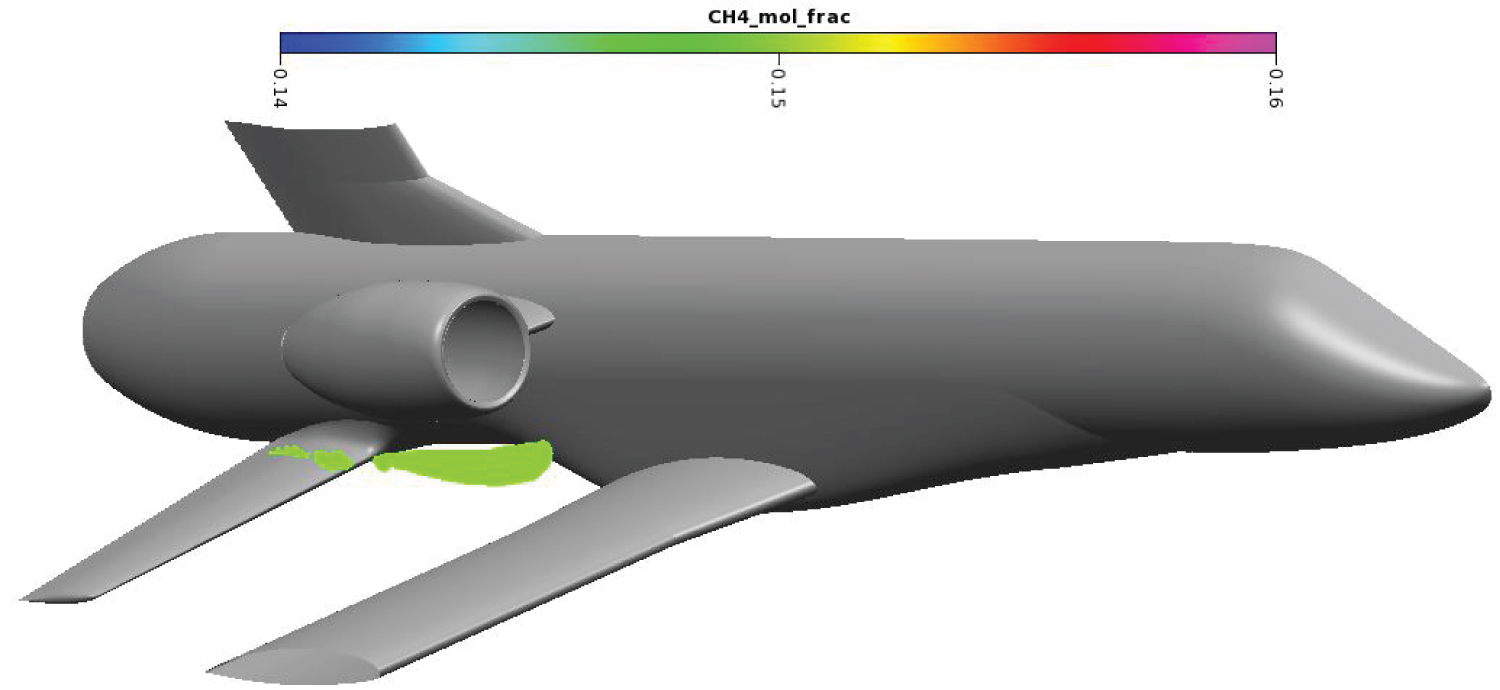
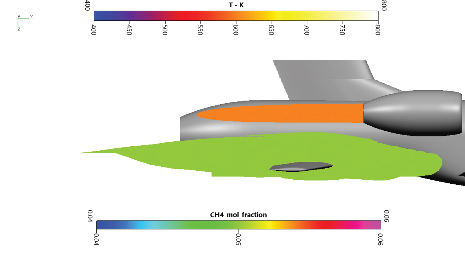
The methane cloud at 15% mole fraction is plotted on Figure 10. Methane in high concentration is located near the draining orifice and stay close to the secondary wing. The methane cloud at 5% mole fraction on Figure 11 is more voluminous. The farthermost part of the cloud extends until the end of the end fairing. Overall, the cloud is more than 6m long and contains around 2.2 m³ of methane in dangerous proportions.

On Figure 12, cutting planes at 30 cm, 4m and 6m behind the draining orifice are presented. The turbojet exhaust temperature and the methane cloud were plotted on these cuts. The first cut being close to the injection, the dangerous zone for methane is shaped like a thin ring. The empty side of the ring denotes an area where methane concentration is above the UFL. The second cutting plane enlightens the fuel cloud on the secondary wing and the temperature from the turbojet exhaust. The cloud lies above and under the secondary wing, possibly creating icing problems on the skin. No mixing is observed with the turbojet hot exhaust. The last cut is located behind the secondary wing, next to the rocket engine fairing. The cloud is less dense, but the dangerous area is still important. There is still no mixing with the exhaust. A low temperature of 600K is chosen on the Figure 12 to highlight there is no mixing between hot combustion gases and methane. Even if mixing was noted, the auto-ignition temperature of 873K is much more important, allowing us to discard auto-ignition in our study.

The methane mole fraction (orange dots) and temperature (blue dots) along a streamline originated from the center of the draining hole are plotted on Figure 13. Using the flammability limits of 5 and 15%, it is possible to delimit the dangerous zone. The temperature inside this zone is under 280 K more than 600 K under the auto-ignition temperature. The dangerous zone is however extensive, meaning that an ignition with an external source could be harmful. Possible sources could be an electrical discharge from lightning or static electricity or an incandescent object coming out of the turbojet. These scenarios were not investigated through CFD, as they required both data on the sources at our flight conditions and extensive computational resources.

Parametric study on the influence of the flight angle

The flight angle has a major influence on the methane trajectory. Three different angles of 0°,4°and 15°were modeled for the same altitude and speed. The plane never flies with a 15° angle while draining but this case is important to notice the trajectory change visually. The draining altitudes are set by the industrial and fixed. No draining can occur during approach for landing or during the climbing phase. In this study, several altitudes were investigated but only the one giving the most constraining results are presented.

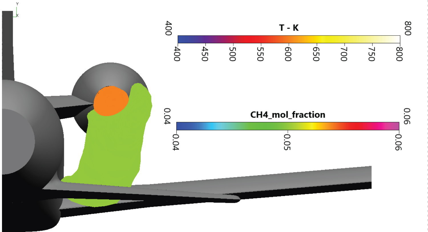
At 0° (Figure 14), the air flow is parallel to the plane centerline. The methane cloud is far from the turbojet flux and surrounds the secondary wing.

At 4° (Figure 15), the cloud is not in contact with the turbojet exhaust but gets closer. The distance the two surface is around 30 cm only. The secondary wing is still surrounded by gaseous methane.

At 15° (Figure 16), some suction is observed on the methane cloud. The fuel mixes completely with the turbojet exhaust and is even in contact with the back end of the pod. In this case, the risk of ignition is very high because of methane concentration and high temperatures.

It is thus fundamental to ensure the draining occurs at small angles.

Conclusion

A simplified way to model the draining of cryogenic liquids from a moving suborbital plane at atmospheric altitude was introduced in this paper. The cryogenic jet was approximated with a densified gas law, which greatly reduced the computational time and lowered the complexity of the model. Draining pressure was increased to conserve liquid density. Experimental validation in a wind tunnel was undertaken and for safety reasons, nitrogen was preferred over methane. A wide range of wind speeds and nitrogen mass flows was explored during the experiments. The wind speed, the nitrogen mass flow rate and pressure, the jet trajectory and the temperature in the tunnel were recorded.

Numerical and experimental results have been confronted for several parameters. Trajectories and liquid columns are accurately modeled by this densified gas law. Within the coldest part of the jet, a gap is noticed between experiments and numerical results. However, good agreement is spotted as soon as the jet warms up a few centimeters after injection. The misty flow observed at the injection is a good analogy of the methane behavior in real conditions. Despite this non-purely liquid jet, the model allows to predict the trajectory in a satisfactory manner, reinforcing the interest of this simplified model. Validation of the model with nitrogen is an important step considering the number of studies on this subject. The use of methane would require a fairly different setup to avoid any risk of explosion and to avoid the release of the gases in the atmosphere.

This model was then applied to the draining of liquid methane from a moving space plane. The ignition risk of the propellant clouds was also investigated. Flammability limits of 5 and 15% in mole fraction were chosen. An important volume of methane in dangerous concentration can be noticed close to the fuselage. This cloud doesn't mix with the turbojet hot exhaust, allowing us to exclude self-ignition possibility. However, an external source such as lightning or static electricity might be able to ignite the propellant.

Thanks to the modularity of the model, dangerous flight conditions can be satisfactorily modeled with a reduced calculation time, which make it relevant for early-stage projects. The results given in the vicinity of the injection should however be considered with care, this model being more accurate farther from the injector. Additional experimental data can be provided by contacting the corresponding author.

Acknowledgements

Support from the CAPRYSSES project (ANR-11-LABX-006–01) funded by ANR through the PIA (Programme d'Investissement d'Avenir) is gratefully acknowledged. Wind tunnel testing was undertaken at the ESA department of PRISME laboratory with the help of Gilles Charles and Stephane Loyer.

References

1. Chochua G, Shyy W, Thakur S, et al. (2000) A Computational and experimental investigation of turbulent jet and crossflow interaction. Numerical Heat Transfer, Part A: Applications 38: 557-572.
2. Kamotani Y, Greberf I (1972) Experiments on a turbulent jet in a cross flow. AIAAJ 10: 1425-1429.
3. Kelso RM, Lim TT, Perry AE (1996) An experimental study of round jets in crossflow. Journal of Fluid Mechanics 306: 111.
4. Smith SH, Mungal MG (1998) Mixing, structure and scaling of the jet in crossflow. Journal of Fluid Mechanics 357.
5. Yuan LL, Street RL (1988) Trajectory and entrainment of a round jet in crossflow. Physics of Fluids 10: 2323-2335.
6. Sykes RI, Lewellen WS, Parker SF (1986) On the vorticity dynamics of a turbulent jet in a crossflow. Journal of Fluid Mechanics 168: 393-413.
7. Esmaeili M, Afshari A, Jaberi FA (2015) Turbulent mixing in non-isothermal jet in crossflow. International Journal of Heat and Mass Transfer 89: 1239-1257.
8. Richards WS, Steinberg AM (2018) Trajectory and breakup of cryogenic jets in crossflow. Journal of Propulsion and Power 34: 269-272.
9. Witlox HW, Harper M, Oke A, et al. (2010) Sub-cooled and flashing liquid jets and droplet dispersion I. Overview and model implementation/validation, Journal of Loss Prevention in the Process Industries 23: 831-842.
10. Elshamy OM (2007) Experimental investigations of steady and dynamic behavior of transverse liquid jets. University of Cincinnati.
11. Faeth G (1991) Structure and atomization properties of dense turbulent sprays. Symposium (Inter- national) on Combustion 23: 1345-1352.
12. Coward H, Jones G (1952) Limits of flammability of gases and vapors. Tech Rep Bulletin 503.
13. Cui G, Li Z, Yang C (2016) Experimental study of flammability limits of methane/air mixtures at low temperatures and elevated pressures. Fuel 181: 1074-1080.
14. Karim G, Wierzba I, Boon S (1984) The lean flammability limits in air of methane, hydrogen, and carbon monoxide at low temperatures. Cryogenics 24: 305-308.
15. Li Z, Gong M, Sun E, et al. (2011) Effect of low temperature on the flammability limits of methane/nitrogen mixtures. Energy 36: 5521-5524.
16. Liaw HJ, Chen KY (2016) A Model for predicting temperature effect on flammability limits. Fuel 178: 179-187.
17. Kundu S, Zanganeh J, Moghtaderi B (2016) A review on understanding explosions from methane- air mixture. Journal of Loss Prevention in the Process Industries 40: 507-523.
18. Bellofiore A, Di Martino P, Lanzuolo G, et al. (2008) Improved modeling of liquid jets in crossflow. ILASS: 8-10.
19. Lee K, Aalburg C, Diez FJ, et al. (2007) Primary breakup of turbulent round liquid jets in uniform crossflows. AIAA Journal 45: 1907-1916.
20. Pai MG, Desjardins O, Pitsch H (2008) Detailed simulations of primary breakup of turbulent liquid jets in crossflow. Tech Rep.
21. Sallam K, Dai Z, Faeth G (2002) Liquid breakup at the surface of turbulent round liquid jets in still gases. International Journal of Multiphase Flow 28: 427-449.
22. Sallam KA, Aalburg C, Faeth GM (2004) Breakup of round nonturbulent liquid jets in gaseous crossflow. AIAA Journal 42: 2529-2540.
23. Strom H, Sasic S, Holm-Christensen O, et al. (2016) Atomizing industrial gas-liquid flows -Development of an efficient hybrid VOF-LPT numerical framework. International Journal of Heat and Fluid Flow 62: 104-113.
24. Kunz O, Wagner W (2012) The GERG-2008 wide-range equation of state for natural gases and other mixtures: An expansion of GERG-2004. Chem Eng Data 57: 3032-3091.
25. Bernard-Champmartin A, Poujade O, Mathiaud J, et al. (2014) Modelling of an homo- geneous equilibrium mixture model (HEM). Acta Applicandae Mathematicae 129: 1-21.
26. (2017) ESI-GROUP, CFD-ACE +
27. Linstrom PJ, Mallard WG (2019) NIST Chemistry Web Book.
28. Wilcox D (1993) Turbulence modeling for CFD. AIAA 93: 2905.
29. Van Doormaal JP, Raithby G D (1984) Enhancements of the simple method for predicting incompressible fluid flows. Numerical Heat Transfer 7: 147-163.
30. Patankar S, Spalding D (1972) A Calculation procedure for heat, mass and momentum transfer in three-dimensional parabolic flows, International Journal of Heat and Mass Transfer 15: 1787-1806.
31. (1976) NOAA U.S. Standard Atmosphere, Tech rep.