Aeroacoustics Analysis of a Dual-Stream Subsonic Jet

Abstract

This work was part of a major investigation for coaxial jet noise prediction and refers to a study of geometrical and velocity parameters and their influence on the noise generated by coaxial nozzles. The Reynolds Averaged Navier-Stokes (RANS) approach coupled with a fluctuation synthetization model and the integral formulation of Curle's Acoustic Analogy were employed to calculate the noise spectrum and compare it to experimental data from JEAN EU project. A sensitivity analysis was carried out by making variations of the secondary to primary stream velocity ratio and the secondary to primary exhaust area ratio. Also, the influence of these parameters in the flow turbulence and noise field were investigated. Encouraging agreement of the predicted far field sound directivity and spectra with measurements was obtained. The noise spectrum was well computed into the range of 100 up to 10000 Hz, corroborating the experimental data by pointing that the lower the secondary to primary velocity ratio and higher the area ratio, the lower the related noise field shall be.

Keywords

RANS, Dual-stream, Jet noise, Acoustic analogy, Velocity ratio, Area ratio

Introduction

Flow from dual-stream (coaxial) nozzles is a field of interest in several engineering applications, such as combustion chambers, cooling systems and pre-mixers among others. However, one the most well-known application is the propulsion system of modern aircrafts by medium and high-bypass turbofan engines. For application of the jet as a way of obtaining thrust for an aircraft, the presence of a secondary stream has prerogatives such as increased thrust (due to the increase in mass flow), more efficient mixing and especially low noise emission [1].

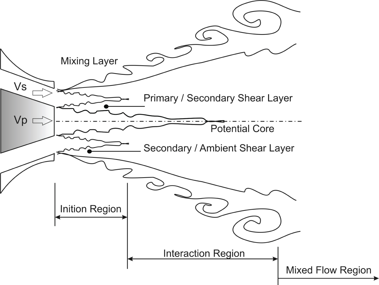
From the physical point of view, the secondary stream (cold-jet) imposed upon a primary flow (hot-jet) brings additional complexity to this turbulent flow as two potential cores must coexist, one central and conical core (primary) and a secondary annular flow. Thus, two shear-layers are also identified: one between the primary and the secondary flow and other between the secondary and the surrounding ambient-flow. Figure 1, as presented by [2] shows this highly-turbulent, three-dimensional and complex flow.

These flow structures are naturally linked to the noise production in a subsonic dual-stream jet, therefore requiring knowledge to describe such turbulent interactions and its correlation with frequency and magnitude. Additionally, the problem with dual-stream jets also presents regions of laminar, transitional and fully turbulent flows. To better know the physics of such problems, several works tried to decompose the flow in distinct regions and associate them with the acoustic signature [2-4] among others.

The problem itself is also governed by external variables which alters the whole flow pattern. The velocity ratio (VR) is one important variable and defines the ratio between the secondary to the primary flow speeds (Vs/Vp). Following the same path, the density ratio (ρ_s/ρ_p) expresses the compressibility effects, and the area ratio (AR) that describes the geometric parameter for the nozzle configuration (A_s/A_p). The AR is an important parameter to indicate the flow pattern [1], mainly the length of the potential core and the spreading rate of the coaxial jet. It is also possible to identify other mixing mechanisms related to the absolute value of flow speeds [5]. Bringing more complexity, there are other variables that influences in a minor or major proportion the fluid dynamics of dual-stream jets and consequently the noise emission: The nozzle thickness, boundary layer development, temperature, boundary conditions such as wind gusts and humidity.

Due to the flow complexity, the aeroacoustics of dual-stream jets is not a straightforward problem to tackle. Still today, one of the major obstacles to predict the acoustic field of coaxial jets is the difficulty to rightly calculate all the fluctuations in the flow field with accuracy in terms of magnitude and frequency [6]. Other authors such as [7], [8] and [9] added relevant information about the flow field and acoustics of dual-stream jets, mainly provided by experimental observations.

With the increasing in the computing power and the speed of data processing, it has been possible to use a direct approach such as DNS (Direct Numerical Simulation) or even LES (Large Eddy Simulation) to evaluate the acoustic fields of jets [10]. This means that the flow field is resolved with enough accuracy to capture even the smallest structures present in the flow in the case of DNS approach or by solving directly the large structures and modeling the minor scales with a sub-grid theoretical model when applying the LES approach. In both cases, the velocity and pressure fluctuations are directly computed and can be converted into an acoustic field anytime. The acoustic information can be propagated to the far field by using acoustic analogies or linearized Euler equations [11]. By following these high-fidelity approaches, Lattice Boltzmann methods were also applied for high-speed non-isothermal jet exhausting from a short-cowl coaxial nozzle [12]. Although these methods are promising for solving the flow field and acoustics with more accuracy, they still have some numerical issues to be tackled and some restrictions in terms of computational resources.

The current work is in the branch of hybrid-approach offering a less costly methodology to solve the aeroacoustics of dual-stream jets. It consists of using RANS coupled to turbulence modelling and a technique to synthetize the fluctuating field. Thus, the method presented was envisaged to serve as a tool to predict and optimize nozzles to be applied in the aeronautical industry. The utilization of hybrid methods has already presented in literature [13] and the synthetization technique also employed for a similar purpose [14]. However, the contribution of this work was to analyze, by using this approach, the influence of velocity ratio (VR) and area ratio (AR) in the noise emission from a coplanar nozzle operating at subsonic speeds. The most important observations were related to the noise reduction found for velocity ratios below 1.0 which are associated to the role of shielding the internal noise sources by the secondary potential core. In that matter, it was possible to see a correlation between noise reduction by decreasing the VR and by increasing the AR. Also, the correlation of the noise emitted by the jet with the external shear-layer development, as well as peak of turbulent kinetic energy was investigated. Although the results were considered satisfactory, it was also possible to identify some flaws and limitations of the method used in the analyzes which are presented and discussed as part of an approach for predicting coaxial jet noise.

Methodology

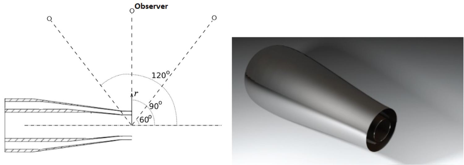
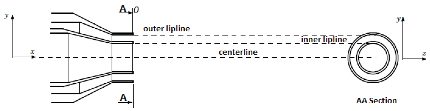
The nozzle geometry used in this study is shown in Figure 2. The coplanar nozzle has been used in the EU JEAN project and in a research collaboration program between ISVR (Institute of Sound and Vibration) and Federal University of Uberlandia following previous works [2] and [15]. For this coplanar nozzle, only acoustic experimental data was available for different area ratio (AR = A_S/A_p): AR = 0.87; 2 and 4; different velocity ratio (VR = V_S/V_p): VR = 0.63; 0.79 and 1.0. One matrix of simulation could be generated according to Table 1, following the nomenclature, as for instance A8V7, which means area ratio 0.87 and velocity ratio 0.79, and so on. It is important to mention that in the database the primary velocity (V_p) was almost constant during the experiments and the secondary velocity (V_s) was varied to achieve the desired velocity ratios.

Hybrid numerical approach

The steady-state flow field has been achieved by employing a RANS (Reynolds Averaged Navier-Stokes equations) approach to solve the three-dimensional (3D) problem of the flow from a subsonic dual-stream jet discharging by a coplanar nozzle with different area and velocity ratios in accordance with Table 1. What is referred to hybrid approach is the fact that the aeroacoustics of the problem is evaluated in two steps: a) Characterization of an averaged flow field by depicting the flow and turbulent variables (source calculation); b) Use of a method or technique to generate the unsteadiness related to the problem (fluctuation of the field); c) Propagation of the noise generated by this field to the location of the observer through a integral propagation solution [16]. It means that the noise signature is not directly calculated by a simple set of equations as described by LES or DNS approach.

Turbulence modeling

The closure turbulence-problem is solved by the use a non-linear k-ε turbulence model, named cubic k-ε model [17]. With the use of this model it is possible to evaluate the averaged fluctuation term $\rho {{\overline{u}}^{\prime }}_{\iota }{{\overline{u}}^{\prime }}_j$, as described below:

$$\begin{array}{l}\rho {{\overline{u}}^{\prime }}_{\iota }{{\overline{u}}^{\prime }}_j={\mu }_t{S}_{ij}+\frac{2}{3}{\delta }_{ik}k+C_1{v}_t\frac{k}{\in }\left(S_{ik}{S}_{kj}-1/3S_{kl}{S}_{kl}{\delta }_{ij}\right)+C_2{v}_t\frac{k}{\in }\left({\Omega }_{ik}{S}_{kj}+{\Omega }_{jk}{S}_{ki}\right)+C_3{v}_t\frac{k}{\epsilon }\left({\Omega }_{ik}{\Omega }_{jk}-1/3{\Omega }_{lk}{\Omega }_{lk}{\delta }_{ij}\right)+\text{ (1)}\\ C_4{v}_t\frac{k^2}{{\in }^2}\left(S_{ki}{\Omega }_{lj}+S_{kj}{\Omega }_{li}\right)S_{kl}+C_5{v}_t\frac{k^2}{{\in }^2}\left({\Omega }_{il}{\Omega }_{lm}+S_{il}{\Omega }_{lm}{\Omega }_{mj}-2/3S_{lm}{\Omega }_{mn}{\Omega }_{nl}{\delta }_{ij}\right)+C_6{v}_t\frac{k^2}{{\in }^2}{S}_{ij}{S}_{kl}{S}_{kl}+C_7{v}_t\frac{k^2}{{\in }^2}{S}_{ij}{\Omega }_{kl}{\Omega }_{kl}\end{array}$$

Where $S_{ij}$ is the rate-of-strain tensor, and ${\Omega }_{ij}$ is the rate-of-rotation tensor. For brevity, the details of formulation in the k-ε cubic model is shortened here. Additional details the reader should consult [17] or other sources like [18] and [19].

Turbulence synthetization

This section describes the main equations for generating a field of synthetic or artificial, velocity fluctuations from a given set of turbulence statistics obtained by the previous RANS formulation. The turbulence synthetization allows a prediction of the acoustics perturbation that can be used as a source term in the wave equation to propagate the perturbation signal until the receptor [10]. In this case, the turbulence synthetization can be used for the generation of full- or part-spectrum synthetic noise sources that can be used with numerical or analytical acoustic wave propagation methods. A synthetic reconstruction of turbulence is attractive because it offers an inexpensive method of generating an unsteady flow field from any localized set of RANS statistics [20,21]. Recent developments for synthesis of turbulence are seen in the work of [22].

In the work of [21] a formulation for a velocity transient field is developed based on previous work of [20]. After, the work of [20] improved the method by avoiding the procedure of finding an orthogonal transformation tensor that would diagonalize a given anisotropic velocity correlation tensor. Details are given to [20].

A new transient field is generated by using Eq. 2. For brevity, a one-dimensional equation is shown:

$${\upsilon }^{*}\left(\overrightarrow{x},t\right)=A_{ik}\sqrt{\frac{2}{N}}{\displaystyle {\sum }_{n=1}^N\left[{\overrightarrow{q}}^n\left({\overrightarrow{k}}^n\right)\cos \left({\widehat{k}}_x^n\cdot \widehat{x}+{\omega }^n\widehat{t}\right)+{\overrightarrow{r}}^n\left({\overrightarrow{k}}^n\right)sen\left({\widehat{k}}_x^n\cdot \widehat{x}+{\omega }^n\widehat{t}\right)\right]}\text{ (2)}$$

where N is the number of Fourier modes, ${\widehat{k}}_x^n$ represents the wave number vector (weighted) in the x-direction.

$$\widehat{x}\text{ = }\frac{2\pi x}{1},\widehat{t}\text{ = }\frac{2\pi t}{1},{\stackrel{⏜}{k}}_x^n\text{ = }\frac{1/\tau }{{\text{c}}^{\text{n}}}\text{ (3)}$$

The turbulent scales of length and the time respectively are represented by l and $\tau$:

$$c^n\text{ = }\sqrt{\frac{3{{\overline{u}}^{\prime }}_{\iota }{{\overline{u}}^{\prime }}_m{\kappa }_l^n{\kappa }_m^n}{2{\kappa }_k^n{\kappa }_k^n}}\text{ (4)}$$

The vectors ${\overrightarrow{q}}^n$ and ${\overrightarrow{r}}^n$ in Eq. 2 are given by:

$${\overrightarrow{q}}^n\left({\overrightarrow{k}}^n\right)\text{ = }{\in }_{ijk}{\overrightarrow{\zeta }}^n{\overrightarrow{\kappa }}^n,{\overrightarrow{r}}^n\left({\overrightarrow{k}}^n\right)\text{ = }{\in }_{ijk}{\overrightarrow{\xi }}^n{\overrightarrow{\kappa }}_k^n\text{ (5)}$$

where ${\in }_{ijk}$ is the permutation tensor used in the vector product operation in Eq. (5). The vectors ${\overrightarrow{\zeta }}^n$ and ${\overrightarrow{\xi }}^n$ are chosen randomly following a normal gaussian distribution.

According to [5] the fluctuations distribution in the jet is slightly different from a gaussian curve.

The variables ${\overrightarrow{\kappa }}^n$ e ${\omega }^n$ represent a sample of n wave-number vectors and frequencies of the modeled turbulence spectrum [21].

$$E\left(\kappa \right)\text{ = 16}{\left(\frac{2}{\pi }\right)}^{1/2}{\kappa }^4\exp \left(-2{\kappa }^2\right)\text{ (6)}$$

Therefore, this method generates a field that does not fulfill the mass conservation equation. Additionally, the generated flow structures stretch in the direction of the main correlation. Due to this reason, it is fundamental to use an anisotropic non-linear turbulence model such as cubic k-ε.

Simulation parameters

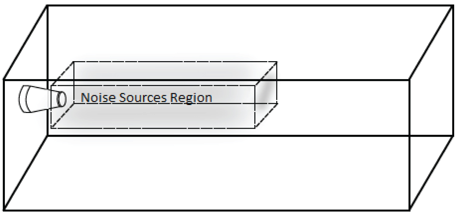
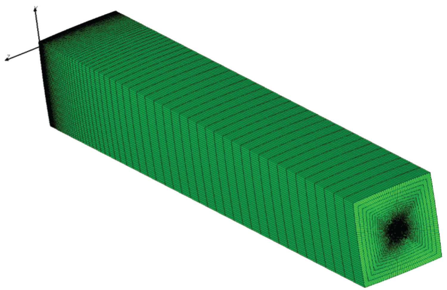
The computational domain has been sized according to [2] as illustrated in Figure 3. The rectangular box has 50 D_s in the streamwise direction (x) and 10 D_s in the (y) and (z).

The far field (infinity) condition was applied in the surrounding faces of the domain by prescribing values of ambient temperature and pressure. The nozzle wall was defined as a non-slip condition. A small velocity value (1 m/s) was adjusted in the left-face of the domain to help the entrainment condition for the coaxial jet near the nozzle. As initial condition, the level of turbulent intensity from the free stream was set to 2% which is achieved close to the mixing layer. Also, the eddy viscosity ratio given by the ratio between the turbulent viscosity and the molecular dynamic viscosity (µ_t/µ) was set to 11, as seen in the work of [23]. Based on this value, the turbulent kinetic-energy and dissipation rate were calculated and prescribed. Inside the nozzle at the respective faces for primary and secondary flow, the stagnation pressure and temperature in accordance with the desired thermodynamic state was imposed. A summary of ambient condition and boundary values for one of the configurations tested in this work is presented in Table 2.

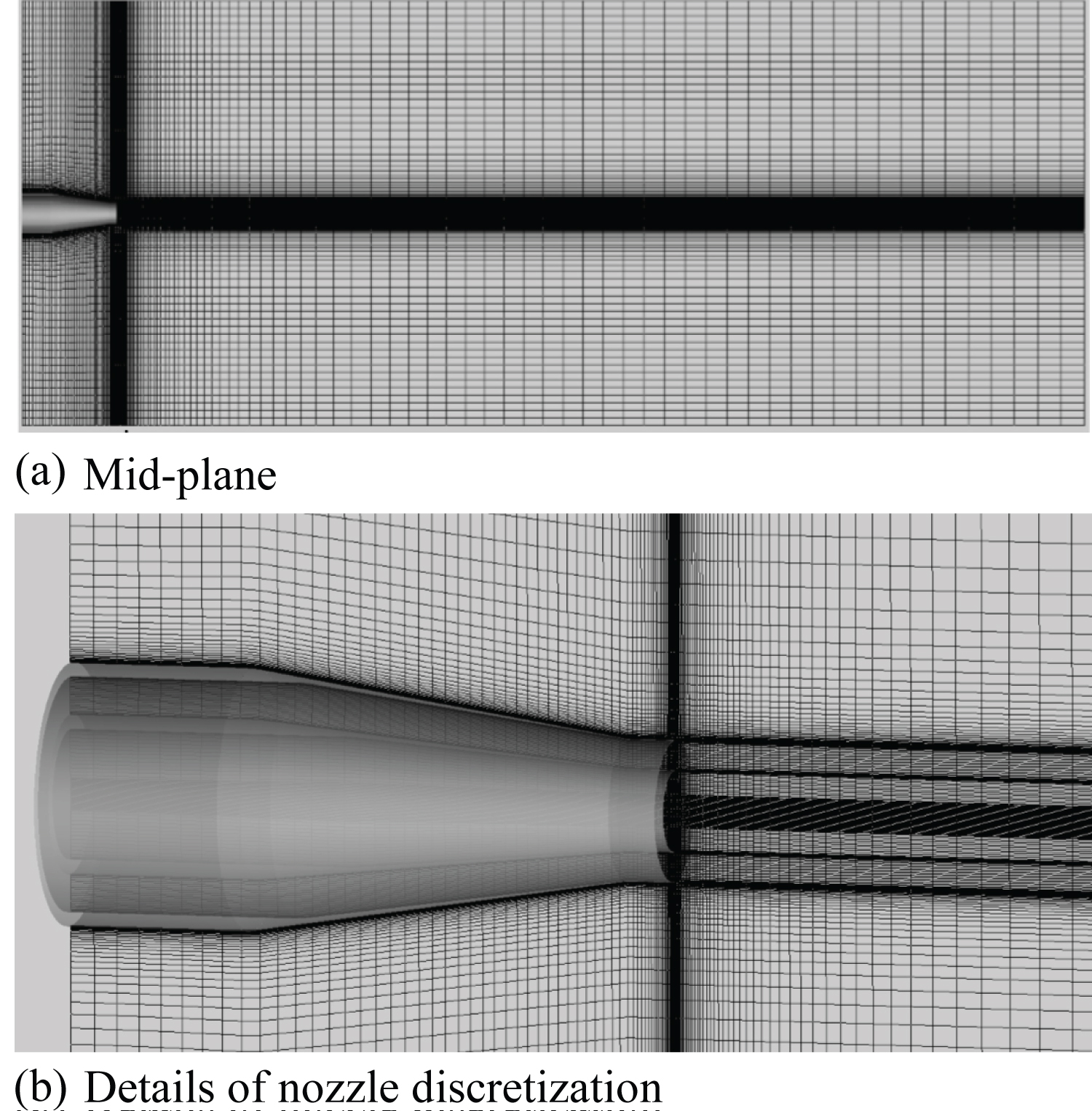
Details of the mesh refinement are given in Figure 4. Mesh refinement is seen close to the nozzle walls to obey the y+ restriction (y+ ≤ 30) in the boundary layer region. A two-layer approach [24] was adopted for solving the RANS equations towards the nozzle walls, which provides reliable results as y+ stays below 300.

Two different mesh refinements were applied to discretize the coplanar nozzle, a first mesh with 3.0 million elements for area ratio of 0.87 and 2.0, and a second mesh with 4.01 million elements for the area ratio of 4.0. Both meshes have a fixed density of elements per domain length, in the proximity of the nozzle is around 1.5 elements for mm of domain extension. Mesh refinement and grid independency study for this class of problem was presented by [2] and [15] and it will be not showed here for brevity. However, it should be mentioned that the number of points per wavelength, as well as the mesh refinement in the nozzle region, has an influence on the results as seen in any type of numerical method. Specifically, for coaxial nozzle simulations, both flow and acoustic fields are dependent of the development of the primary and secondary shear-layers as well the jet's spreading which could be improved with more attention to mesh refinement. Thus, it is believed that in this work the mesh refinement was consistent with the configurations to be analyzed, providing at the same time reliable results and good leading time.

Noise propagation to far field

Once the synthetization procedure had reconstructed the fluctuating velocity field for a calculated set of turbulence statistics the resulting acoustic pressures as a function of position (x_i) and time (t) could be evaluated following the volumetric integral acoustic analogy as the Curle's formulation [16], also used by [11]. A solution to Curle's equation, which is valid for arbitrary r can be written as (see, for example, [25]):

$$p^{\prime }\left(x_i,t\right)\text{ = }\frac{1}{4\pi }{\displaystyle \int {\displaystyle \int {\displaystyle \int \left[\frac{l_i{l}_j}{a_0^{2}R}\frac{{\partial }^2{T}_{ij}}{\partial t{}^2}+\frac{3l_i{l}_j-{\delta }_{ij}}{a_0^{2}r}\frac{\partial T_{ij}}{\partial t}+\frac{3l_i{l}_j-{\delta }_{ij}}{R^3}{T}_{ij}\right]}}}d\overrightarrow{Y}\text{ (7)}$$

where $R\text{ = }\left|\overrightarrow{X}-\overrightarrow{Y}\right|$ and T_ij is the stress tensor of Lighthill [6]. The Eq. (7) is already simplified to only account for the quadrupoles sources associated to the fine-scale turbulent fluctuations. Therefore, Eq.(7) was solved in a "tuned" adjusted mesh that is a rectangular volumetric region defined as source region in Figure 3, and illustrated in Figure 5, as an example.

Fluid Dynamics Results

The acoustic field is intrinsically related to the fluid dynamics and a good prediction of the dual-stream jet will lead to satisfactory noise spectra. Due to limitation of space, only part of the fluid dynamics results is presented in this section, covering, as example, radial profiles of u-velocity, axial normalized velocity-profile in the jet centerline and radial profiles of turbulent intensity.

The profiles were extracted in the radial direction at normalized location y/D_s and in the longitudinal direction x/D_s, corresponding to the centerline of the jet, as described in Figure 6.

The results in sequence were obtained in a machine with 8 Intel® Core™ i7-3930K CPU @3.20GHz processors, 24 Gbytes of RAM memory and operational system of 64 bits, taking approximately 60 hours of computation.

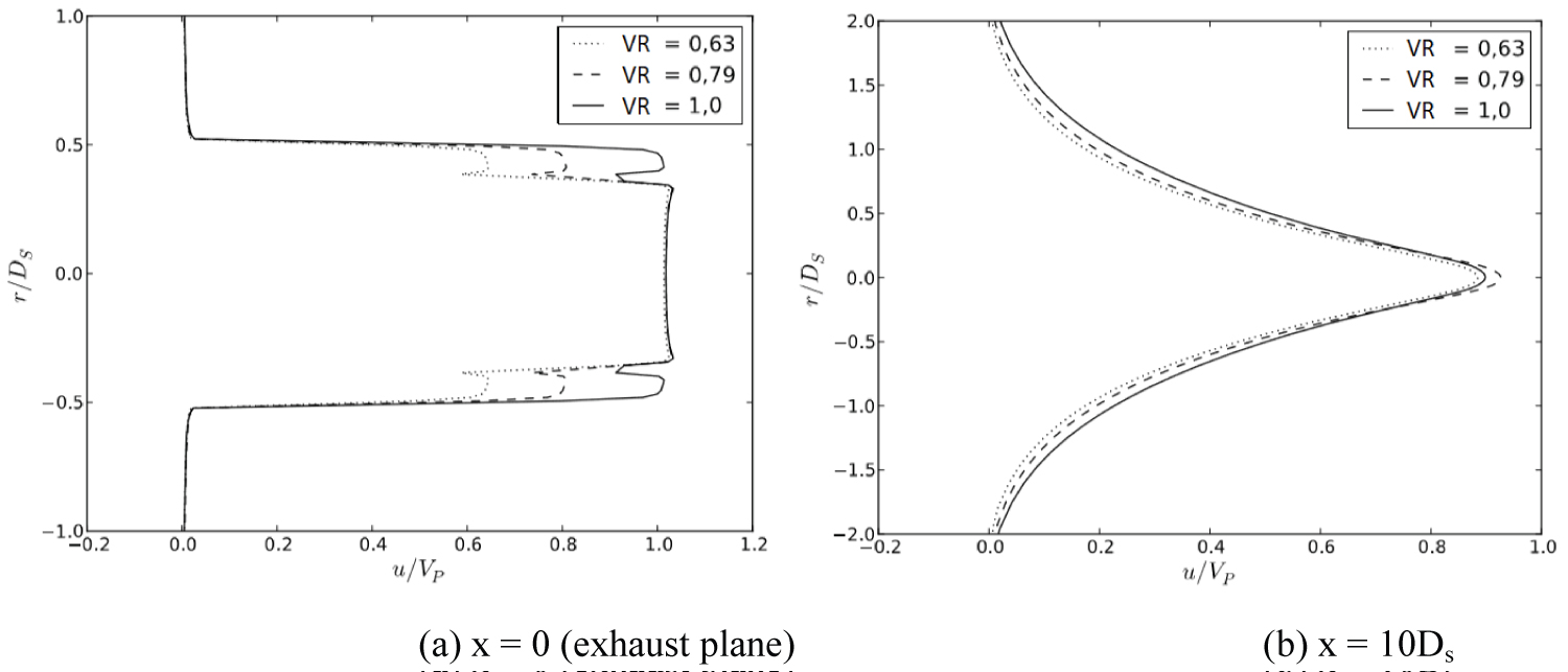
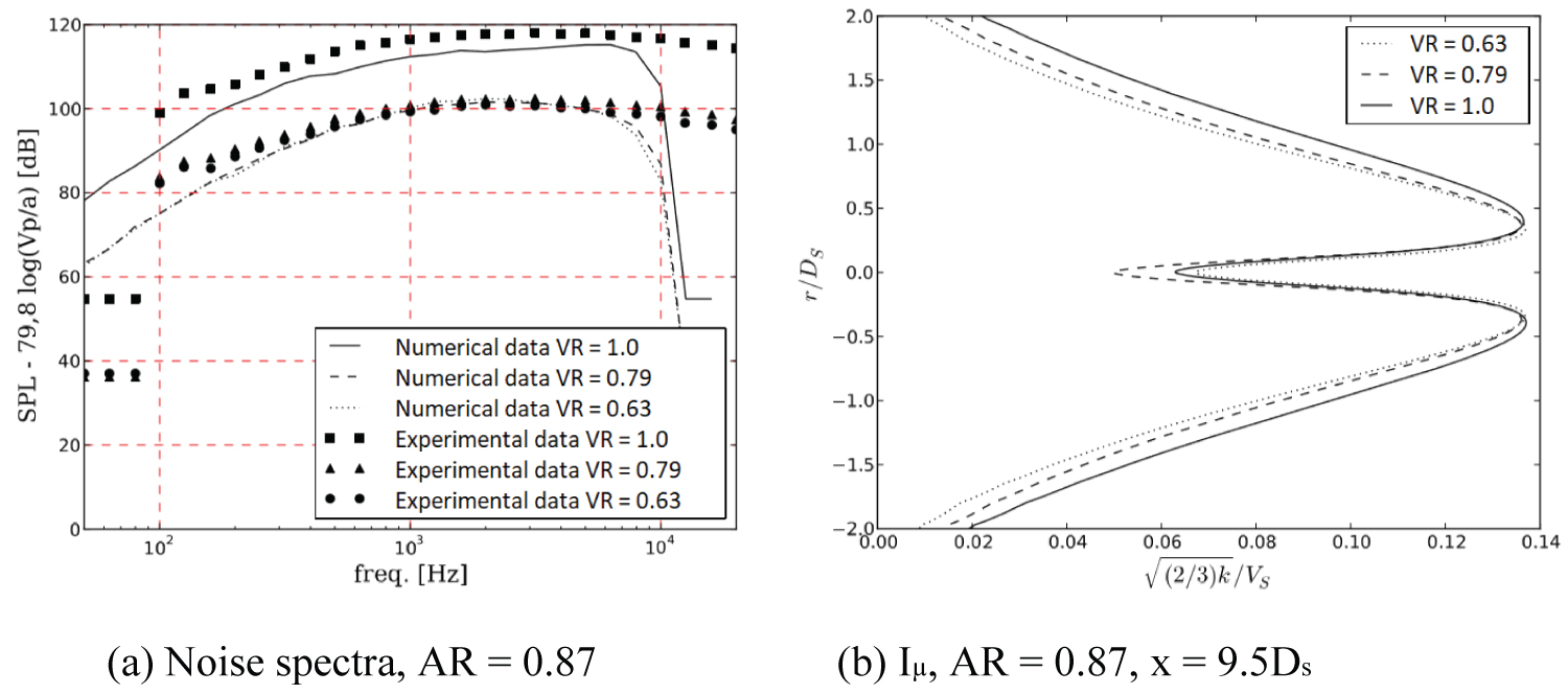
Figure 7 shows the radial profiles of u-velocity for an area ratio of 0.87 with three different velocity ratios (VR = 0.63; 0.79 and 1.0). The potential core is extinguishing approximately at x ≈ 10D_s (position where the velocity at the centerline reaches approximately 95% of the primary velocity). Moreover, for the velocity ratio of 0.79 the potential core is slightly bigger when compared to VR = 0.63 and 1.0.

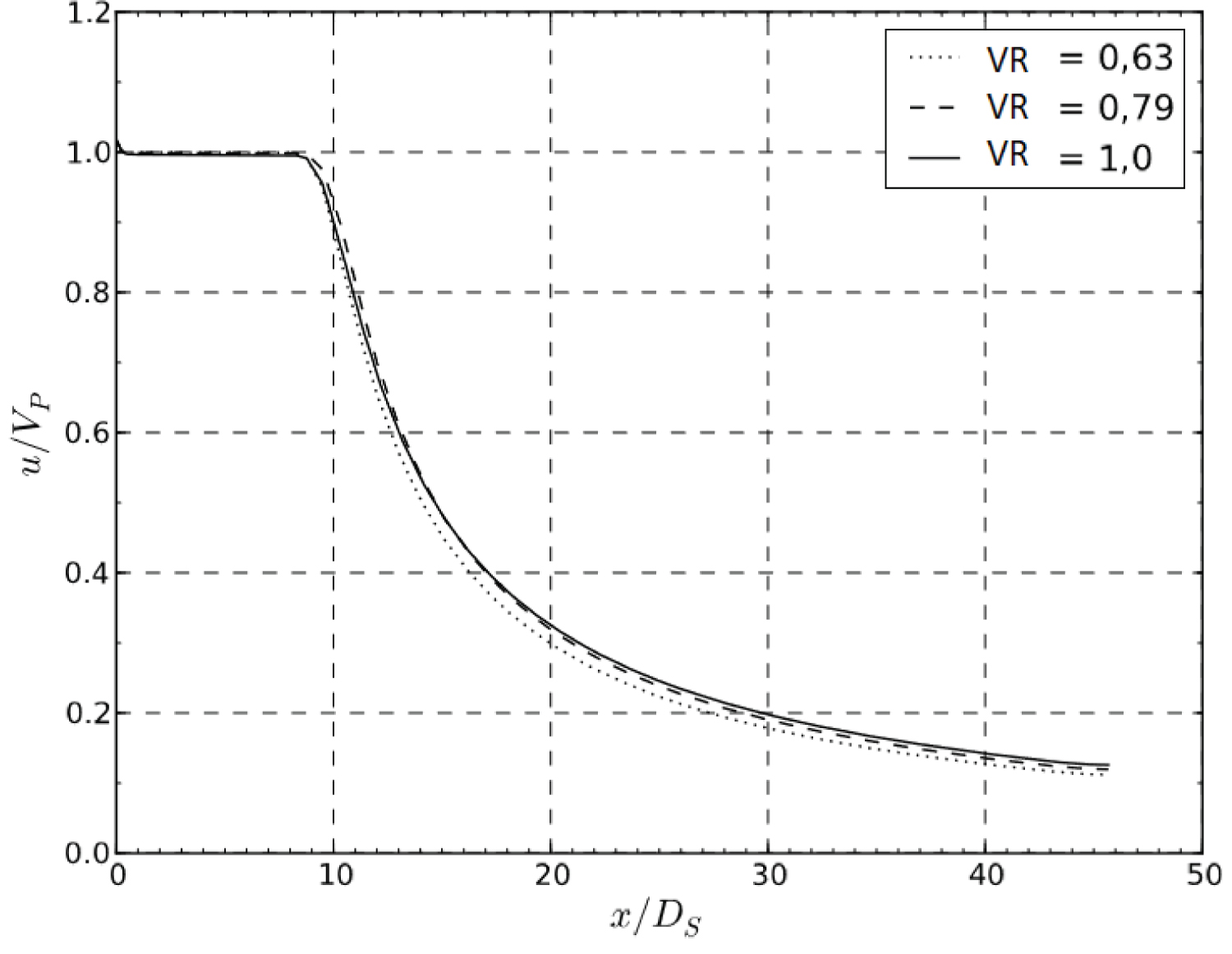
The influence of the velocity ratio on the potential core length and decaying rate is almost negligible. Figure 8 corroborates this observation, where calculated potential core length was around 10 D_s.

Based on previous calculation with coaxial nozzles, described in the works of [2] and [15], it is possible to affirm that this kind of numerical approach generally overpredicts the length of the potential core. It is believed that in the jet centerline the actual size of the potential core is around 9D_s.

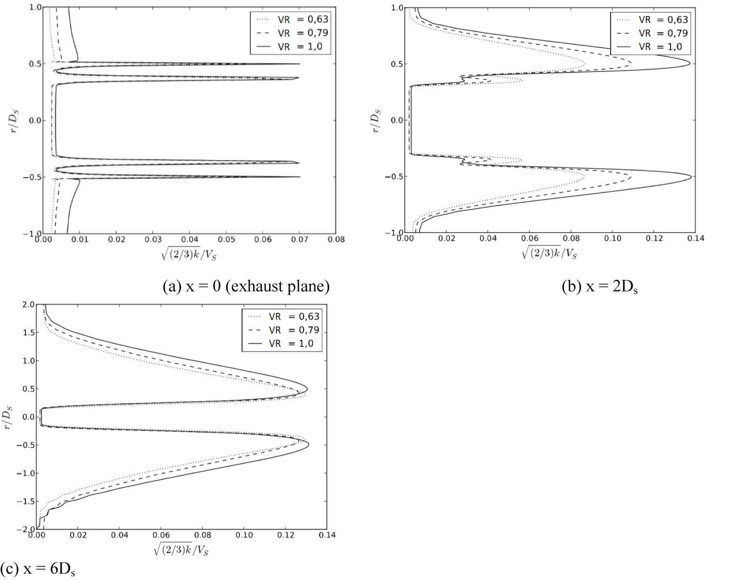
Figure 9 presents the radial profiles of turbulent-intensity, according to Eq. (8) for an area ratio of 0.87.

$$I_{\mu }\text{ = }\frac{\sqrt{\frac{2}{3}k}}{V_p}\text{ (8)}$$

As the secondary velocity is increased (high values of VR), the primary shear-layer has lower values of turbulent intensity, while in the secondary shear-layer the levels are higher in comparison. Although not all results are shown here, it can be stated that flow velocity field for AR = 2.0 and 4.0 is very similar to the field for AR = 0.87 except for the variation of the secondary potential core length.

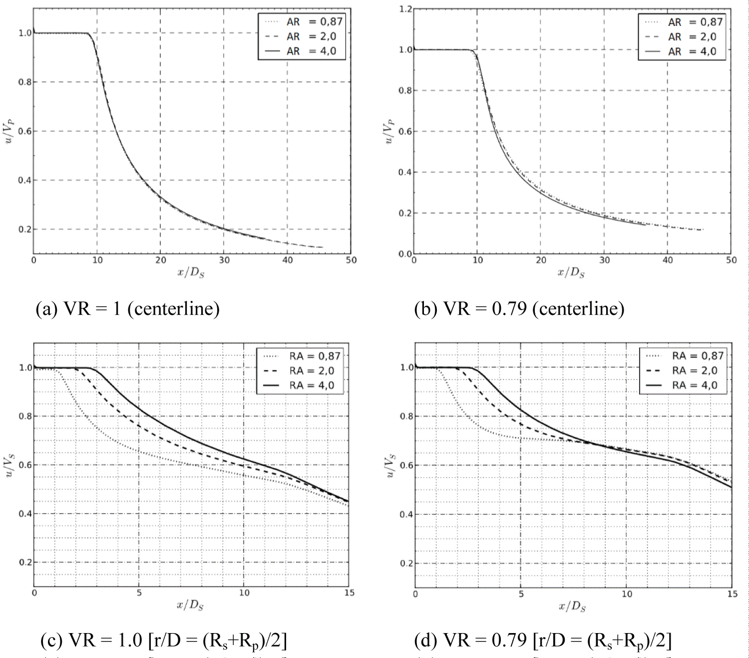
In Figure 10 the axial profiles of u-velocity in the centerline extracted in the radial position (R_s + R_p)/2 (centerline of the secondary jet), which is expected to demonstrate the length of this secondary-stream. To complete this analysis, in Figure 10a and Figure 10b it is illustrated the length of the primary-stream, which is slightly variable with the area ratio.

The length of the secondary potential core is elongated with higher values of AR and it is nearly unalterable with the VR (at least in the cases investigated).

Experimental data from [5] indicates that for a coaxial-jet configuration with VR = 0.8 and AR = 5.2, the secondary potential core extinguishes before 2 D_s. According to Figure 10 it is observed that for a VR = 0.79 and AR = 4.0, this length was around 3.5 D_s. The prediction of the secondary potential core length is particularly important due to the shielding phenomenon that may reduce the noise emission.

Aeroacoustics Results

After the flow field calculation, with the averaged velocities and turbulent quantities k and ε, it was employed the synthetization technique for obtaining the fluctuation field and getting the acoustic field associated. In this section the noise spectra are presented for the cases studied. Again, due to limitation of space part of the results are shown. Additional details could be left to [15]. All the acoustics results have been obtained with a time step of Δt = 5.0 × 10^-5 s, a sampling time of 1.5 s, totalizing 30000 time steps with a Fourier number of 100. It is important to emphasize that several parameters associated to this methodology has been tested in [15].

To summarize the set of results, only three angular positions are presented, respectively: 60°, 90° and 120°. The synthetization technique and propagation procedure took about 38 hours, in average, to conclude. Thus, a complete simulation (fluid dynamics and acoustics) totalized approximately 100 hours (4 days) of computing.

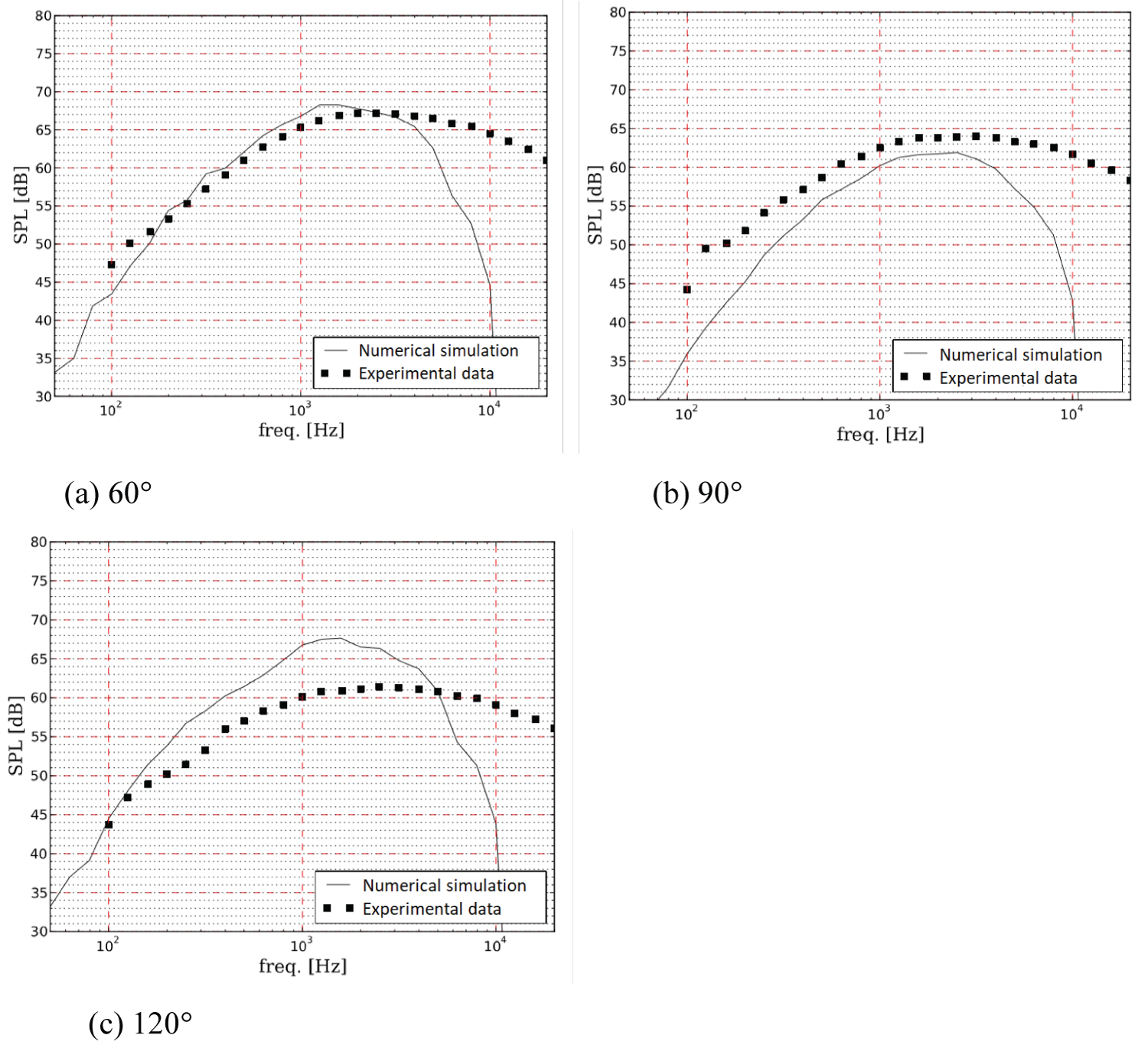
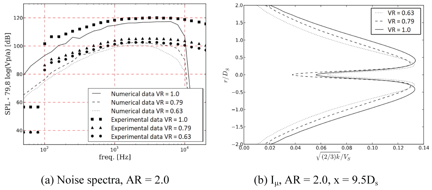
Figure 11 illustrates the comparison of numerical and experimental data in terms of noise spectra for the configuration VR = 0.63 and AR = 2.0. The observer location for each polar angle was respectively: $\left|\overrightarrow{X}\right|$ = 11.9 m (60°), $\left|\overrightarrow{X}\right|$ = 12.9 m (90°) and $\left|\overrightarrow{X}\right|$ = 13.5 m (120°).

The experimental data available was in the frequency range of 100 up to 40000 Hz while the numerical was adjusted to have a cut-off frequency around 5000 Hz. This was due to the size of the volumetric elements used in the calculation procedure, which at the end reflects the number of points per wavelength.

In Figure 11 two important aspects could be identified. The first one was related to the SPL levels at 90°, which in this case was underpredicted by the simulation. As well-known at this observer location it is expected a close agreement to the experimental data since the sound propagation is almost free of refraction effects (not completely embedded in this methodology). Even though the result did not match completely the spectrum the trend was well-captured. Another point was related to the noise prediction at shallow angles such as 60°. In this case the result was closer to the experimental data with a slightly overprediction in the medium part of the spectrum (~1000 Hz). As pointed by [8], high sound pressure levels are expected for lower angles of observation, evidencing the preferred directivity of the jet. Possible drawbacks of this methodology showed by the deviation of the peak levels for 90° were associated to the reconstruction of the turbulent field under the refraction effects. It is also believed that more points per wavelength would result in a better agreement with the experimental data. Moreover, as pointed in section 4, the generated flow structures have the tendency of stretching in the direction of the main correlation in turbulent synthetization technique, what could be influencing the results. Such limitation could be tackled by correcting or improving the turbulence model for dealing with such aspect of the flow field more properly.

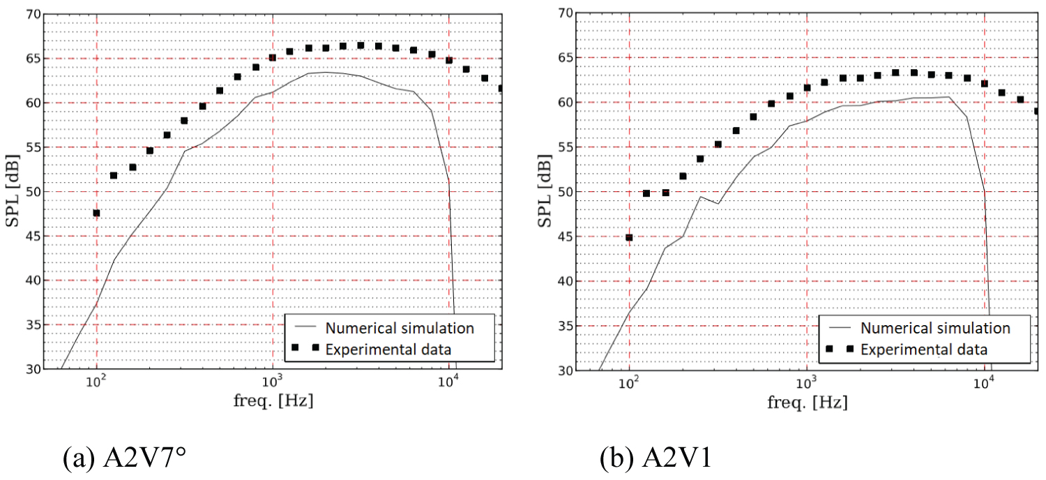
Although some discrepancies were seen between numerical and experimental data for the configuration A2V6, the simulations were extended for the other configurations: A2V7 and A2V1; as presented in Figure 12. It was observed that the levels are still underpredicted varying from 2 dB at higher frequencies and reaching in the worst conditions at lower frequencies values around 10 dB. The same trend was observed for the other configurations showed in Table 1 and simulated in this work.

It is also important to emphasize that the primary velocity (V_p) was kept almost constant among the simulations, in accordance to the experimental data, only varying the velocity of the secondary-stream. Thus, as pointed by Figure 11b the levels are lower when compared to Figure 12a, because of lower turbulent intensity levels in the shear-layer of the coaxial jet. On the other hand, for the configuration A2V1, the experimental data showed a lower primary velocity when compared to other configurations. This discrepancy has made the direct comparison a little more difficult.

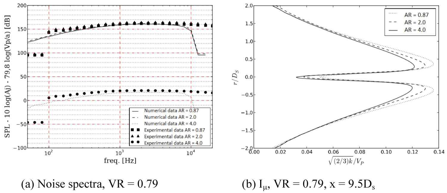
As a completion of this work, the entire Table 1 was simulated, and the data compared against the experimental data. Values of diameters and exhaust velocities were modified in manner to understand the influence of these parameters. However, it is important to note that the mass flow information was not considered in this analysis. The noise reduction to be effective should keep the mass flow rate to the nozzle (directly proportional to the thrust). This parameter was not considered. Thus, to proceed with a comparison between configurations and to determine if there was effective noise reduction, normalization as proposed by [8] was considered, following the equation:

$$SP{L}^{*}\text{ = }SPL-10\log \left(A_j\right)-79.8\log \left(\frac{V_p}{a}\right)\text{ (9)}$$

According to the configuration, by applying Eq. (9) to the data it is possible to infers if there was noise reduction or not, as a function of area and velocity. Figure 13, Figure 14 and Figure 15 illustrate these normalized data showing noise reduction related to the velocity ratio. The presence of a secondary-stream promotes a substantial decrease in noise, the lower the velocity ratio, better is the gain in terms of reduction, as has been identified before. In the same figure, the turbulent intensity plots were included as data correlation.

As visualized in Figure 13, Figure 14 and Figure 15, the noise reduction was quite similar for all area ratios.

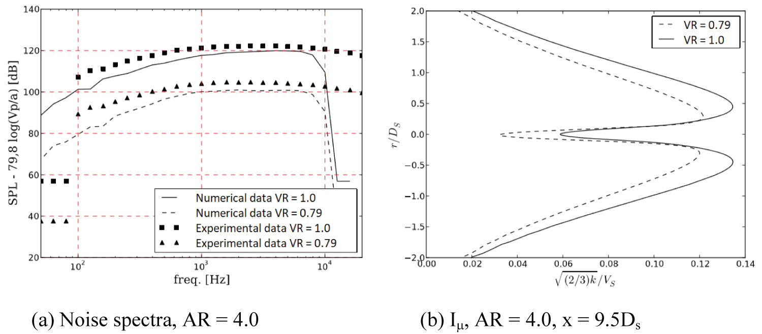
In Figure 16 and Figure 17, it is possible to observe a noise reduction associated to an AR = 4.0. Even though the noise levels were under predicted (at least for an observer at 90°), the trends were well captured. The noise variation between area ratios of 0.87 and 2.0 were not noticeable, according to Figure 13 and Figure 14, since the exhaust area was kept the same, according to $\left(A_s+A_p\right)\text{ = }\pi {\text{D}}_s^2/4$ with D_s = 0.058 m.

Conclusion

In this work the fluid dynamics parameters and noise spectra from a coplanar nozzle operating at subsonic speeds were addressed. A supposed computationally low-cost methodology was considered, providing a complete analysis in a timeframe of 40 h, considering the availability of a previous well-computed steady flow field. The Randon Flow Generation technique was applied with some adjustments to generate an instantaneous and fluctuating turbulent field as sound source.

Based on the results, it was possible to state that there was no linear proportionality between the velocity ratio and the levels of turbulent intensity. For all area ratio investigated, there was no pattern for the variation in the velocity ratio, as the intermediary values of VR have presented lower levels of turbulent intensity in the central region of the jet. More detailed experimental data including more variations of VR could help to explain such kind of confirmation.

It was also possible to affirm that the cubic k-ε turbulence model had deficiencies for predicting turbulent quantities with low level of shear, giving possibly underestimated turbulent levels. As a consequence, the length of both primary and secondary potential core was overestimated which implies in a dislocation of the region with more turbulent activity in the jet for downstream.

For velocity ratios below 1.0 it was identified a relatively noise reduction. This may be related to the increase in the length of the secondary potential core, what helps the mixing process and plays a role of shielding the internal noise sources. A lengthier secondary potential core is preferred when is desirable a lower noise emission. It was possible to affirm that there was correlation between noise reduction by decreasing the VR and by increasing the AR. The noise emitted by the jet, for all simulation, seemed to be correlated with the external shear-layer, as well as the peak of turbulent kinetic energy, found at the end of the primary potential core.

The methodology used in this work was not completely able to predict low-frequency noise, with deviation of about 10 dB. However, it is expected that with mesh refinement and tuning of more points per wavelength an improvement in the results. The noise pattern found in the results agreed with information from literature, pointing out that the bigger the AR lower is the noise and the lower the VR less noise is emitted, at least for the investigated cases in the range VR = 0.63 up to 1.0.

To establish the current methodology as a tool for assisting the design of nozzles with low noise emission, more work could be done in the direction of improving the Randon Flow Generation technique by including spatial correlations to avoid vortex-stretching and uncorrelated sources, as well as increasing the size of points per wavelength (mesh refinement) putting the cut-off frequency as high as possible.

For future and on-developing works, it is proposed a better approach with more sophisticated non-linear turbulence models, study and improvement of initial conditions and augmentation of the computational power, which are flaws of the current methodology.

Acknowledgements

The first author thanks the financial support provided by CNPq - Conselho Nacional de Desenvolvimento Científico e Tecnológico for the development of this work. Also, we thank Prof. Aristeu da Silveira Neto for all support in MFLAB (Fluid Mechanics Laboratory).

References

1. E Murakami, D Papamoschou (2002) Mean flow development in dual-stream compressible jets, AIAA Journal 40: 1131-1138.
2. Almeida (2009) Aeroacoustics of Dual-stream Jets with Application to Turbofan Engines. Ph.D. thesis, Dept. Aeronautical Eng., Technologic Institute of Aeronautics, S. José dos Campos, BR.
3. LEM Lima (2007) Análise Numérica de Jatos Coaxiais Turbulentos. Ph.D. thesis, National Institute of Spatial Research., S. José dos Campos, BR.
4. MJ Fisher, GA Preston, WD Bryce (1998) A modelling of the noise from simple coaxial jets, part I: With unheated primary ?ow. Journal of Sound and Vibration 209: 385-403.
5. R Sadr, JC Klewicki (2003) An experimental investigation of the near-field ?ow development in coaxial jets. Physics of Fluids 15: 1233-1246.
6. MJ Lighthill (1952) On sound generated aerodynamically I. General theory. Proceedings of the Royal Society of London A 211: 564-587.
7. DJ Bodony, SK Lele (2005) Generation of low frequency sound in turbulent jets. 11^th AIAA/CEASA Aeroacoustics Conference (26^th AIAA Aeroacoustics Conference).
8. K Viswanathan (2004) Aeroacoustics of hot jets. Journal of Fluid Mechanics 516: 39-82.
9. CKW Tam, K Viswanathan, KK Ahuja, et al. (2008) The sources of jet noise: Experimental evidence. Journal of Fluid Mechanics 615: 253-292.
10. Markesteijn AP, Gryazev V, Karabasov SA, et al. (2020) Flow and noise predictions of coaxial jets. AIAA Journal 1-14.
11. M Billson, LE Eriksson, L Davidson (2005) Acoustic source terms for the linearized Euler equation in conservative form. AIAA American Institute of Aeronautics and Astronautics Journal.
12. Casalino D, Lele SK (2014) Lattice-Boltzmann simulation of coaxial jet noise generation. In Proceedings of the Summer Program 231-240.
13. RH Self, A Basseti (2003) A RANS based jet noise prediction scheme. 9^th AIAA/CEAS Aeroacoustics Conference and Exhibit.
14. L Davidson, M Billson (2006) Hybrid LES-RANS using synthesized turbulent ?uctuations for forcing in the interface region. International Journal of Heat and Fluid Flow 27: 1028-1042.
15. FGT Ferreira (2013) Análise Aeroacústica de Jatos Coaxiais em Regime Subsônico. Ms.C. dissertation, School of Mechanical Eng., Federal University of Uberlândia, Uberlândia, BR.
16. N Curle (1955) The in?uence of solid boundaries upon aerodynamic sound. Prog. R. Soc. Lond., Manchester, England.
17. G Easom (2000) Improved turbulence models for computational engineering. Ph.D. thesis, University of Nottingham.
18. TJ Craft, BE Launder, K Suga (1996) Development and application of a cubic eddy-viscosity model of turbulence. International Journal of Heat and Fluid Flow 17: 108-115.
19. SB Pope (1975) A more general effective-viscosity hypothesis. J Fluid Mech 72: 331-340.
20. R Kraichnan (1970) Diffusion by a random velocity field. Phys Fluid 13.
21. A Smirnov, S Shi, I Celik (2001) Random ?ow generation technique for large eddy simulations and particle-dynamics modeling, Journal of Fluids Engineering 123: 359-371.
22. T Auerswald, A Probst, J Bange (2015) An anisotropic synthetic turbulence method for large-eddy simulation. Int. Journal of Heat and Fluid Flow 62: 407-422.
23. A Dauptain, B Cuenot, LYM Gicquel (2010) Large eddy simulation of stable supersonic jet impinging on ?at plate. AIAA Journal 48: 2325-2338.
24. W Rodi (1991) Experience with Two-Layer Models Combining the k-e Model with a One-Equasion Model Near the Wall. 29^th Aerospace Sciences Meeting.
25. J Larsson (2002) Computational aero acoustics for vehicle applications. Ph.D. thesis, Chalmers University of Technology, Göteborg, Sweden.