Predicted Accelerations of Surface-Mounted Electron Devices during Spacecraft Launch
Abstract
Nonlinear dynamic response of a thin-and-flexible horizontally-oriented rectangular printed circuit board (PCB), whose non-deformable support contour is subjected to a suddenly applied constant acceleration during spacecraft vertical launch, is considered. The general concept is illustrated by a numerical example. It is shown that the accelerations of the board's inner points could be much higher than the acceleration of its support contour. The results of the analysis could be used, particularly, when deciding if the acceleration-sensitive electron devices are robust enough and where to place them on the board, so that the induced acceleration will still be below the allowable level.
Keywords
Spacecraft launch, Printed circuit board, Nonlinear dynamic response, Constant acceleration, Non-deformable support contour, Acceleration-sensitive-electron-devices
Introduction
Elevated accelerations could possibly cause mechanical and/or functional failures of the surface-mounted electron devices. Dynamic response of electronic and photonic systems to shocks and vibrations was addressed in numerous publications (see, e.g., [1-10]). In this analysis the nonlinear dynamic response of a spacecraft PCB, with surface-mounted IC devices on it, is considered and analyzed. The spacecraft vertical launch condition is addressed, and the engineering theory of bending of plates is employed to analyze the response of a thin-and-flexible board, whose non-deformable support contour experiences a suddenly applied constant acceleration during spacecraft launch. The objective of the analysis is to predict the accelerations at inner points of the board. These accelerations might exceed significantly the acceleration of the board's support contour. The cases of simply supported and clamped boards are considered. The analysis is an extension and a modification of the author's earlier work [2,3]. The current (for the past five years or so) state-of-the-art could be found in numerous NASA website information and publications.
Analysis
Stress function
Consider a printed circuit board (PCB) whose non-deformable support contour experiences suddenly applied and constant vertical acceleration (Figure 1). Using the engineering theory of thin plates (see, e.g., [11,12]), the normal in-plane stresses and and the shearing stress in the board could be expressed through the stress (Airy) function φ(x,y) as follows:
The function φ(x,y) should satisfy the continuity equation
Where, w = w(x,y,t) are the board's deflections, E is Young's modulus of its material, and the bi-harmonic operator ∇4 and the operator L are
In the case of a non-deformable contour, the function φ(x,y) must satisfy also the conditions
Where υ is Poisson's ratio of the board's material, and a and b are the board's dimensions in the x and y directions, respectively. These conditions indicate that, for a non-deformable contour, the in-plane displacements caused by the in-plane ("membrane") tensile stresses and should be equal to the displacements caused by the board's bending. The conditions (4) are based on assumptions that the board's material is isotropic and homogeneous.
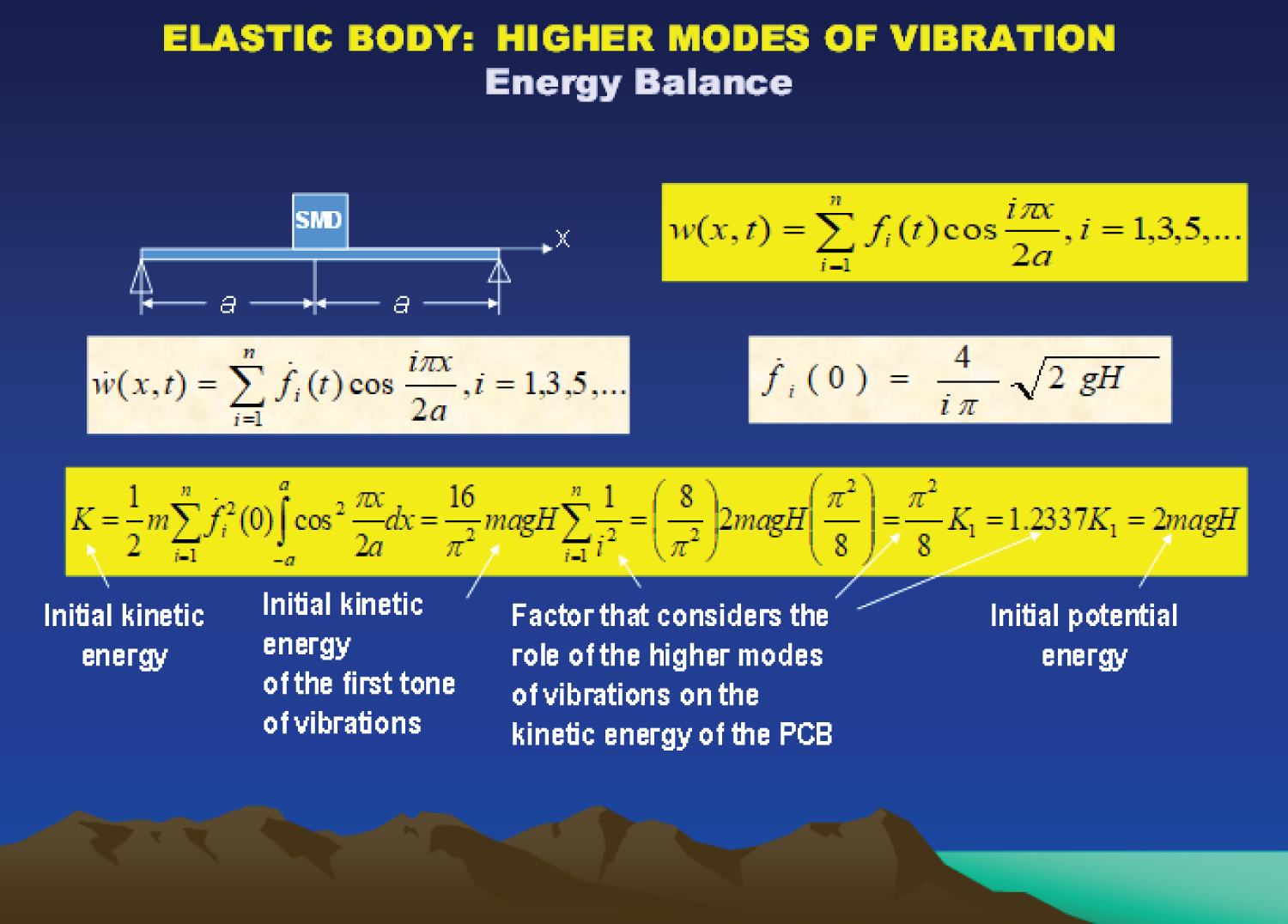
Our analysis is limited to the first mode of vibrations. The derivation in Figure 2 justifies such a limitation even for a linear system, in which the role of the higher modes is expected to be considerably higher than in a nonlinear system, mostly because the strain energy of the first mode of vibrations in linear systems does not contain the energy caused by the in-plane strains, which result in nonlinear effects. The situation, when the surface mounted device is mounted on an elongated PCB, is addressed, and it is shown that, as far as the kinetic energy of the PCB experiencing shock-excited linear vibrations is concerned, the higher modes represent only about 23% of the total PCB energy. When deflections are significant and the board's vibrations become nonlinear, this percentage is even smaller, so that, in an approximate analysis, consideration of the first mode of vibrations seems to be justified.
So, the functions w = w(x,y,t) and φ(x,y) could be sought as
Here wc(t) is the vertical displacement of the board's support contour, w1(x,y) is the coordinate function of the first mode of vibrations, z(t) is the corresponding principal coordinate, and φ1(x,y) is the static (time independent) stress function.
In the case of a simply supported board, one could put
Substituting (5), with consideration of (6), into the continuity equation (2) and into the conditions (4) of non-deformability of the board's support contour, we conclude that that the function φ1(x,y) should satisfy the equation
And the conditions
Then the following expression for the static stress function φ1(x,y) could be obtained:
For a square board (a = b) this formula yields:
Although the situation might be much more complicated for a clamped board [13] experiencing nonlinear vibrations, in an approximate analysis it could be assumed that for a clamped board, whose aspect ratio is between 1.0 and 1.5, one could put [14,15],
This leads to the following expression for the static stress function φ1(x,y):
For a square board this formula yields:
Equation of motion
The kinetic, T, and the strain, V, energies of the board are expressed as (see, e.g., [11,12])
Here A = ab is the board area, m is its mass per unit area (with consideration of the masses of the mounted components, assuming that, in an approximate analysis, these masses can be uniformly spread out over the board's surface), is the board's flexural rigidity (we assume that the sizes of the mounted components are small, and therefore they affect only the board's mass, but not its flexural rigidity), h is the board's thickness, and is the Laplace operator. The first term in the second formula in (14) is due to bending, and the second term is due to the tensile membrane stresses.
Substituting (5) into (14), the following formulas for the kinetic and the strain energies can be obtained:
Here
Introducing the formulas (15) into the Lagrange equation (see, e.g., [14])
We obtain the following nonlinear differential equation for the principal coordinate z(t):
Where
is the excitation force caused by the acceleration of the board's support contour,
is the factor that considers the effect of the coordinate function on the magnitude of this force, and is the vertical displacement of the support contour. For a simply supported board
For a square simply supported board (a = b)
For a clamped board
For a square clamped board (a = b)
Note that the parameter α of non-linearity is a little higher for a clamped board than for a simply supported one. For v = 1/3, e.g., the ratio of these parameters for square boards is 1.306.
Maximum deflection, velocity and acceleration
The maxima of the deflection, velocity and acceleration can be determined even without solving the equation (18) of motion (this is always useful, of course, and is done in Appendix A). Indeed, the equation (18) can be written as
Hence, the expression in the parentheses (which is, in effect, the total energy of the board) should be constant:
If the initial displacement and the initial velocity are zero, the constant C should be zero as well, so that the equation
Should be fulfilled. This equation, written as
Determines the s. c. phase diagram, which establishes the relationship between the displacement and the velocity for the given nonlinear system.
The maximum value zmax of the displacement takes place for ż = 0 and, as evident from (27) and (28), can be found from the cubic equation
Its solution is
Where
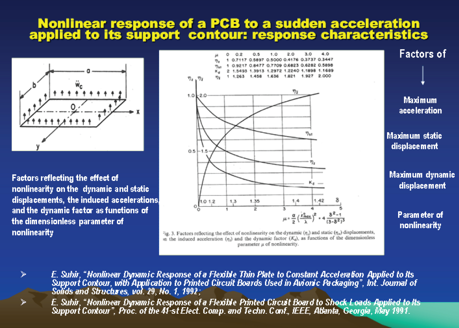
Is the maximum linear dynamic displacement (α = 0), and the factor ηz that considers the effect of the nonlinearity on the maximum nonlinear dynamic displacement could be obtained from the equation (29) as
Where
Is dimensionless parameter of nonlinearity of the dynamic system in question. The factor ηz tends to one, when the parameter µ of nonlinearity tends to zero. It will be shown in the Appendix that the exact solution to the basic equation (18) leads to a different dimensionless parameter of nonlinearity,
As follows from the formulas (33) and (34),
When μ changes from zero to infinity, δ changes from 1 to . Some further details could be found in the Appendix. Note that in Figure 1 both governing parameters μ and δ are indicated.
The maximum linear static displacement can be found from (18) by putting and and is
Comparing this result with (31), we conclude that the dynamic factor for the maximum linear displacement is If the same suddenly applied constant load q is applied to a linear system dynamically and stays on this system, the induced maximum displacement is twice as large as the displacement, when this load is applied statically. In a linear system this is also true for the maximum velocity and the maximum acceleration, but in a nonlinear system, as will be shown below, the effect of nonlinearity is different for the displacements, velocities and accelerations, and, as far as the accelerations are concerned, could be significantly greater than in a linear system.
The maximum nonlinear static displacement zst. can be found from (18) by putting This leads to the following cubic equation
For this displacement. This equation has the following solution:
Where the factor
Considers the effect of non-linearity on the maximum static displacement. The dynamic factor is in this case
It decreases from for a linear system (α = 0, μ = 0) to Kd = 1 for a highly nonlinear system.
The initial acceleration of the board points can be obtained from (18) by putting the displacement z(t) equal to zero. This, considering (19), yields:
The formula (20) indicates that the factor c is, in effect, the dynamic factor for the maximum initial acceleration. This factor is equal to for a simply supported board and is just slightly higher, , for a clamped board.
The distribution of the induced accelerations over the board's surface can be obtained from the first formula in (5) as follows:
As evident from this formula, the initial acceleration is the maximum on the board's contour (where w1 = 0) and is the minimum
At its center, where w1 = 1. In the case of a simply supported board, using (6), we have:
This formula indicates that the initial accelerations are negative within the rectangular
The minimum acceleration in the center of the board, in accordance with (43), is, for a simply supported board, . In the case of a clamped board, whose coordinate function is expressed by the formula (11), the initial acceleration is Thus, negative initial accelerations occupy a rather large portion of the board area and their absolute maxima are comparable with the magnitude of the acceleration of the board's contour. In elongated boards the region of the negative initial accelerations is -0.212a ≤ x ≤ 0.212a for a simply supported board, and -0.169a ≤ x ≤ 0.169a for a clamped board. The accelerations at the board center for a simply supported and clamped boards are and , respectively.
As one could see from the basic equation (18), the induced acceleration of the board becomes zero, when the displacements become equal to their static values z = zst. At this moment of time all the points of the board have the same acceleration as its support contour. At the end of the first quarter-period of board's vibrations, when the board reaches its maximum deflection z = zmax, its acceleration, as follows from (18), is
Since the induced velocity is zero at this moment of time, the formula (27) yields:
Introducing this relationship into (46), we have:
This equation can be written as
For the linear maximum acceleration and the maximum displacement. Here is the dynamic factor for the maximum acceleration in the nonlinear system and is the dynamic factor for the maximum displacement in such a system. The maximum acceleration in a linear system can be found from (46) by putting
Introducing this expression into (49) and solving the obtained equation for the factor we have:
From (31) we have:
Introducing this product into (49) we obtain the following simple relationship between the dynamic factor for the nonlinear acceleration and the dynamic factor ηz for the nonlinear displacement:
The calculated response characteristics (dynamic factors) are shown in Table 1. As evident from the calculated data, nonlinearity can result in a significant increase in the induced accelerations.
The absolute (total) accelerations of the board at the moment of time equal to the quarter period of vibrations are
As evident from this formula, all the points of the board have at this moment of time the same directions of their maximum accelerations, as the board's support contour. At the center of the board they are by a factor of
Larger than on the board's support contour. In a linear system this factor is η0 = 1 + c = 2.621 for a square simply supported board, η0 = 2.273 for an elongated simply supported board, η0 = 2.778 for a square clamped board, and η0 = 2.165 for an elongated clamped board. In a strongly nonlinear system, when the dynamic factor of the induced acceleration approaches 3.0, the factor η0 for the total acceleration at the center of the board reaches η0 = 5.863 in the case of a square simply supported board, η0 = 4.819 in the case of an elongated simply supported board, η0 = 6.334 in the case of a square clamped board, and η0 = 4.495 in the case of an elongated clamped board. This information is summarized in Table 2.
These data indicate that there is an incentive for using elongated, rather than square boards, and that non-linearity might have a significant effect on the maximum accelerations in the mid-portions of the board. It is clear that in a situation, when the IC or photonic devices are mounted on both sides of the board, the devices and their interconnections on the convex (lower) surface of the board are in the worse situation than those on the concave (upper) side of the board, because the board's surface on its convex (lower) side is subjected to tension caused both by the reactive tension and the board bending. It is noteworthy also that because of the structural damping the vibrations will fade in the course of time, and therefore at the moments of time sufficiently remote from the moment of loading, the board's accelerations will not be different of the accelerations of its contour.
Numerical Example
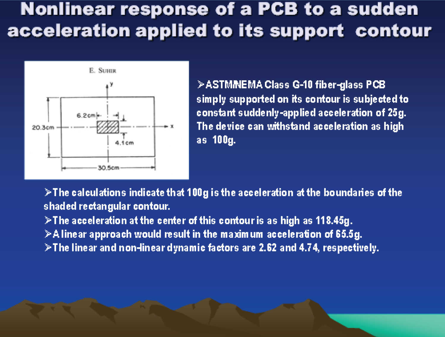
Let an ASTM/NEMA Class G-10 fiber-glass PCB simply supported on its contour be subjected to a constant suddenly applied acceleration applied to its contour. Let the weight of all the surface-mounted devices are 20% of the board's weight, and let there exists certain flexibility in the location, where the given device could be mounted on the board. The device cannot safely withstand accelerations exceeding 100 g. Let us determine, where this device could be safely installed, so that its reliable operation and strength are not compromised. We use the following input data: density of the PCB material: ; Young's modulus: ; Poisson's ratio: v = 0.3; thickness: h = 1.59 mm; dimensions: a = 203 mm; b = 305 mm; And here is the calculated data: Frequency of the free linear vibrations of the board: λ = 463.5 s-1; Parameter of non-linearity: α = 12.3 × 106 cm-2s-2; Force acting on the PCB contour: q = 39715 cms-2; Maximum linear dynamic displacement: ; Non-dimensional parameter of non-linearity: ; Factor considering the effect of non-linearity on the maximum displacement: The maximum non-linear displacement is . Factor considering the effect of non-linearity on the maximum acceleration: ; The distribution of the total (absolute) maximum acceleration over the board's surface predicted by the formula (42) is
Where, g is the acceleration due to gravity.
The condition results in the following equation for the rectangular that restricts the region, within which the device cannot be mounted: . Thus, the device/package should be placed, for safe operation, outside the region shown in Figure 3. The maximum acceleration at the center of the board is . Note that the linear approach would predict the following maximum acceleration at the PCB center: and would result in an erroneous conclusion that the device could be safely mounted anywhere on the board.
Conclusions
The following conclusions can be drawn from the carried out analyses:
1) Simple, easy-to-use and physically meaningful analytical model has been developed on the basis of the engineering theory of thin plates for the evaluation of the induced accelerations in a flexible PCB in a spacecraft during its launch.
2) It is shown that the accelerations of the inner points of the board could be significantly higher than of those on its support contour and that, for an immovable support contour, it is important to account for the nonlinearity of the board's vibrations.
3) The results of the analysis could be used particularly, when deciding where to place acceleration sensitive electron devices on the board. They can also be used when designing experiments and to build the most appropriate test vehicle.
4) The supporting structure could have some components to absorb vibration as well, e.g., dynamic vibration absorber technique. Such a possibility will be considered as a future work.
5) The results of the analysis could be used when designing a suitable experiment, conducting computer-aided simulations, considering, if necessary, the appropriate absorber techniques, and, if there is a need, to optimize the structure for the anticipated loading conditions.
References
- Steinberg DS (1973) Vibration analysis of electronic equipment. John Wiley, New York.
- Suhir E (1992) Response of a flexible printed circuit board to periodic shock loads applied to its support contour. ASME J App Mech 59: S253-S259.
- Suhir E (1992) Nonlinear dynamic response of a flexible thin plate to constant acceleration applied to its support contour, with application to printed circuit boards used in avionic packaging. Int J Solids and Structures 29: 41-55.
- Suhir E (2002) Could shock tests adequately mimic drop test conditions? ECTC Proc.
- Heand X, Stallybrass M (2002) Impact response of a printed wiring board. International Journal of Solids and Structures 39: 5979-5990.
- M Amabili (2004) Nonlinear vibrations of rectangular plates with different boundary conditions: Theory and experiments. Computers and Structures 82: 2587-2605.
- Suhir E, Arruda L (2009) The coordinate function in the problem of the nonlinear dynamic response of an elongated printed circuit board (PCB) to a drop impact applied to its support contour. European Journal of Applied Physics 48.
- Suhir E, Arruda L (2010) Could an impact load of finite duration acting on a duffing oscillator be substituted with an instantaneous impulse? Journal of Solid Mechanics and Materials Engineering 4.
- Suhir E, Steinberg D, Yi T (2011) Dynamic response of electronic and photonic systems to shocks and vibrations. John Wiley.
- Suhir E (1997) Is the maximum acceleration an adequate criterion of the dynamic strength of a structural element in an electronic product? IEEE CPMT Transactions, Part A 20.
- Timoshenko SP, Woinowski-Krieger S (1969) Theory of plates and shell., McGraw-Hill, New-York.
- Suhir E (1991) Structural analysis in microelectronic and fiber optic systems, vol.1, basic principles of engineering elasticity and fundamentals of structural analysis. Van Nostrand Reinhold, New York.
- Levy S (1942) Bending of rectangular plates with large deflections. NACA TN.
- Levy S (1942) Square plate with clamped edges under normal pressure producing large deflections. NACA TN.
- Pars LA (1965) A treatise on analytical dynamics. Heinemann, London.
- Bateman H, Erdelyi A (1955) Higher Transcendental Functions, McGraw-Hill, NY.
- Abramowitz M, Stegun IA (1964) Handbook of mathematical functions with formulas, graphs and mathematical tables. Applied Mathematics Series, National Bureau of Standards, Washington, DC.
Corresponding Author
E Suhir, Bell Laboratories, Physical Sciences and Engineering Research Division, Murray Hill, NJ; Departments of Mechanical and Material and Electronic and Computer Engineering, Portland State University, OR, USA; Department of Applied Electronic Materials, Institute of Sensors and Actuators, Technical University, Vienna, Austria; James Cook University, Mackay Institute of Research and Innovation, Townsville, Queensland, Australia; ERS Co., 727 Alvina Ct., Los Altos, CA 94024, USA, Tel: 650-969-1530; 408-410-0886.
Copyright
© 2020 Suhir E. This is an open-access article distributed under the terms of the Creative Commons Attribution License, which permits unrestricted use, distribution, and reproduction in any medium, provided the original author and source are credited.