Model Predictive Filtering Based Neural Networks for GPS GDOP Approximation

Abstract

This paper presents a new method to calculate the geometric dilution of precision (GDOP) of GPS by incorporating the concept of model predictive filtering in the training process of neural networks to learn the relationship between GDOP and the azimuth and elevation of satellite. This method overcomes the shortcomings of the traditional back propagation neural networks, such as the slow convergence speed and easily falling into local minimum. A model predictive filtering algorithm is developed by using network weights as system state variables to optimize the network weights based on the neural network's error correction. During the training process, the neural network model error is corrected by compensating the deviation between the actual and target output via the model predictive filtering. Experimental results and comparison analysis demonstrate that the proposed method can effectively approximate GDOP with improved accuracy and reduced training time.

Keywords

Neural network, Model predictive filtering, Weight training, GDOP approximation

Introduction

GPS is a commonly used sensor in dynamic vehicle navigation. Its navigation accuracy is heavily dependent on the geometric dilution of precision (GDOP). GDOP is a geometrically determined factor, which is important to the layout design of a satellite-based navigation system [1-3]. It describes the geometric effect on the relationship between measurement error and position determination error, and its value is related to the number and geometric layout of satellites in navigation positioning [4,5].

The most straightforward approach to obtaining GDOP is to compute the trace of the measurement matrix inversion and then select the minimum one, which is called the matrix inversion solution (MIS). However, MIS presents a computational burden to the navigation processor [6,7]. Due to its strong robustness, non-linear fitting, self-learning ability and easy implementation, neural network has received great attention in the area of satellite navigation to process the satellites information (azimuth and elevation) and further calculate GDOP values [8,9]. This method can approximate any complex nonlinear relationship and its learning rule is easy to implement [10]. One of the earliest studies was reported by Simon and El-Sherief, where a back-propagation neural network (BPNN) was developed to learn the functional relationship between the measurement matrix and its inverse eigenvalues to obtain GDOP values [11]. As the training of weights is conducted by minimizing the error function via gradient descent, it suffers from the problem of local minimum. The computation of gradient descent is also expensive, as each iteration involves a time-consuming process of line search. Tafazoli and Mosavi developed a recurrent wavelet neural network (RWNN) to compute GDOP, where the activation function uses gradient steepest descent to improve the learning speed and network reliability [12]. However, due to the similar learning process as BPNN, the RWNN also suffers from the problem of local minimum. Hamed, et al. reported a feed-forward neural network training method based on principal component analysis and Levenberg-Marquardt (LM) to classify GPS GDOP [13]. However, this method still suffers from the local minimum problem, due to the use of gradient descent in the Levenberg-Marquardt optimization. Tabatabaei and Mosavi analyzed the performances of different neural network configurations and training methods based on GLONASS measurements, and further developed a genetic algorithm (GA) to optimize the neural network weights [14]. However, the performance of the genetic algorithm relies on how to effectively guide the mutation operator. Li, et al. reported a new method using general regression neural network (GRNN) for GDOP approximation, where the training samples were selected and normalized using spectrum analysis [15]. However, it causes an expensive computational load in the case of multiple-layer structure. In general, with most of the existing neural network models for GDOP estimation, the training process suffers from various problems such as the slow convergence speed, local minimum, and disturbance of sudden changes in the signals [16].

Model predictive filtering (MPF) is a method to determine minimum model error during the estimation process, where the model error is not limited to Gaussian noise characteristics [17]. This method estimates the model error by comparing actual outputs with measurements, and subsequently remedies the filtering conditions according to the model error to obtain the system state estimation. Due to the real-time performance in the estimation and correction of model error, MPF is capable of handling large and dynamic errors of a nonlinear system, leading to a continuous solution without discrete jumps in system state estimation [18,19].

This paper adopts the concept of MPF for the first time to the network training process to optimize network weights based on the correction of the neural network model error. Based on this, it further presents a new MPF-based neural network method for GDOP approximation. By treating the network weights as system state variables, the model predictive filtering is established to optimize the network weights based on correction of the neural network model error. Different from the BPNN method that conducts the training of weights by minimizing the error function via gradient descent and involves the time-consuming line search at each iteration, the proposed MPFNN method provides an optimal estimation mechanism for training of network weights with fast convergence speed, thus overcoming the BPNN limitations such as the local minimum problem and the expensive computation of gradient descent. Experimental results and comparison analysis have been conducted to comprehensively evaluate the performance of the proposed MPFNN method for GDOP approximation.

Model Predictive Filtering Based Neural Network

Model predictive filtering

Consider the nonlinear system

$$\widehat{\dot{x}}(t)=f(\widehat{x}(t))+G(\widehat{x}(t))D(t)\left(1a\right)$$

$$\widehat{y}(t)=h(\widehat{x}(t))\left(1b\right)$$

where $\widehat{x}(t)\in R^n$ is the state estimate vector, $f\in R^n\to R^n$ is sufficiently differentiable, $G(\widehat{x}(t)):R^n\to R^{n\times q}$ is the model error distribution matrix, $D(t)\in R^q$ represents the model error vector, $h(\widehat{x}(t))\in R^n\to R^m$ is the measurement vector, and $\widehat{y}(t)\in R^m$ is the estimated output vector.

Following (1b), the discrete measurement equation can be represented as

$${\tilde{y}}_k=h(x(t_k))+v_k\left(2\right)$$

where ${\tilde{y}}_k\in R^m$, x(t_k) and $v_k\in R^m$ represent the measurement vector, true state vector and measurement noise vector at time t_k, respectively.

Assume that v_k is a Gaussian white noise process [20] with zero mean and

$$E\left[v_k\right]=0,E\left[v_k{v}_j^T\right]=R{\delta }_{kj}\left(3\right)$$

where $R\in {\text{R}}^{m\times m}$ is a positive-definite measurement covariance matrix.

By Taylor series, the output estimate in (1b) can be expanded as

$$\widehat{y}(t+\Delta t)\approx \widehat{y}(t)+\text{S}(\widehat{x}(t),\Delta t)+\text{Λ}(\Delta t)\text{U}(\widehat{x}(t))D(t)\left(4\right)$$

where the i^th element of $\text{S}(\widehat{x}(t),\Delta t)$ is given by

$${\text{S}}_i(\widehat{x}(t),\Delta t)={\displaystyle \sum _{k=1}^{p_i}\frac{\Delta t^k}{k!}}{L}_f^k(h_i)\left(5\right)$$

where p_i (i = 1, 2, ….. m) is the lowest order of the derivative of $h_i(\widehat{x}(t))$, and $L_f^k(h_i)$ is the k^th-order Lie derivative [19]. $\text{Λ}(\Delta t)\in R^{m\times m}$ is a diagonal matrix with elements given by

$${\lambda }_{ii}=\frac{\Delta t^{p_i}}{p_i!},i=1,2,\cdots ,m\left(6\right)$$

$\text{U}(\widehat{x}(t))\in R^{m\times q}$ is a matrix with each of the i^th rows described by

$${\text{U}}_i(\widehat{x}(t))=[L_{g1}{L}_f^{p_i-1}(h_i),\cdots ,L_{gq}{L}_f^{p_i-1}(h_i)],i=1,2,\cdots ,m\left(7\right)$$

The cost functional is constructed by adding the weighted sum of squares of the residuals between the measurements and estimates and the weighted sum of squares of the model correction terms together

$$\begin{array}{l}J(D(t))=\frac{1}{2}{[}^{(}{R}^{-1}[(t+\Delta t)-\widehat{y}(t+\Delta t)]+\\ \frac{1}{2}{D}^{\text{T}}(t)\text{A}D(t)\left(8\right)\end{array}$$

where $\text{A}\in {\text{R}}^{q\times q}$ is the weighting matrix of the model error and generally obtained by empiricism.

It is assumed that we have a constant sampling rate such that ỹ(t+Δt) ≡ ỹ_k+1. Substituting (4) into (8) and minimizing (8) with respect to D(t) yield the following model error solution:

$$D\left(t\right)=-{\left\{{\left[\Lambda \left(\Delta t\right)U\left(\widehat{x}\left(t\right)\right)\right]}^T{R}^{-1}\left[\Lambda \left(\Delta t\right)U\left(\widehat{x}\left(t\right)\right)\right]+A\right\}}^{-1}$$ $${\left[\Lambda \left(\Delta t\right)U\left(\widehat{x}\left(t\right)\right)\right]}^T{R}^{-1}\left[S\left(\widehat{x}\left(t\right),\Delta t\right)-\tilde{y}\left(t+\Delta t\right)+\widehat{y}\left(t\right)\right]\left(9\right)$$

Using the matrix inversion lemma [21], the model error in (8) can be rewritten as

$D(t)=-\text{M}(t)[\text{S}(\widehat{x}(t),\Delta t)+\widehat{y}(t)-$ỹ$(t+\Delta t)]\left(10\right)$

where

$\begin{array}{l}M\left(t\right)={\left\{{\left[\Lambda \left(\Delta t\right)U\left(\widehat{x}\left(t\right)\right)\right]}^T{R}^{-1}\left[\Lambda \left(\Delta t\right)U\left(\widehat{x}\left(t\right)\right)\right]+A\right\}}^{-1}\cdot \\ {\left[\Lambda \left(\Delta t\right)U\left(\widehat{x}\left(t\right)\right)\right]}^T{R}^{-1}\left(11\right)\end{array}$

In the model predictive filtering, (10) is used in (1a) to nonlinearly propagate the state estimate at time t_k. Subsequently, the measurement at time t_k+1 is processed to find the new D(t) in, [t_k, t_k+1] and the state estimate is further propagated to time t_k+1.

MPF based neural network training

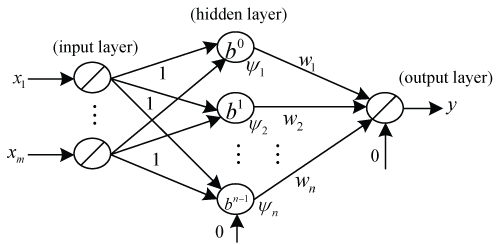
In order to optimize the network weights by MPF, based on the polynomial interpolation and approximation theory, this paper establishes a new neural network structure by setting the excitation function as a group power function of gradually increased order and letting the network parameters be ingenious.

As shown in figure 1, the neural network structure includes the following components: x_i represents the value of the ith input neuron; Ψ_j is the output of the j^th hidden neuron; and w_j denotes the interconnection weight between the j^th hidden and output neurons.

The net internal activity of hidden neurons is given by

$$b={\displaystyle \sum _{i=1}^m{x}_i}\left(12\right)$$

where b is the sum of the inputs to all the neurons on the hidden layer.

The output of the j^th neuron is computed by

$${\psi }_j(b)={({\displaystyle \sum _{i=1}^m{x}_i})}^{j-1}\left(13\right)$$

where $j\in [1,n]$

The output of the entire neural network is computed by

$$y={\displaystyle \sum _{j=1}^n{w}_j\cdot }{\psi }_j(b)\left(14\right)$$

In this neural network structure, both the input and output layers adopt an identical linear function as the activation function, while the hidden layer uses a group power function of gradually increased order (namely, the activation function of the j^th hidden layer is in the j-1^th order of the input: Ψ_j(b) = b^j-1, (j = 0,1,2,---, n-1). For the simplification purpose, the threshold value for all neurons in the neural network structure is set as zero and the weights between input and hidden layer are set as one.

The optimization of the weight matrix w can be treated as a minimization problem of weighted least squares, where the model error vector is the difference between the neural network's actual output and target output.

Consider neural network architecture with m inputs, n hidden units and one output. Define the target output as y and the actual output at time t as

$$y={[y_{11},\cdots ,y_{1Q}]}^T$$

$$h(\widehat{x}(t))={[{\widehat{y}}_{11},\cdots ,{\widehat{y}}_{1Q}]}^T\text{ (15)}$$

where Q is the number of training samples.

By associating the weights with the system state, the state of the nonlinear system can be represented as

$$w={[w_1\cdots w_n]}^T\left(16\right)$$

Further, by associating the neural network output with the output of the nonlinear system, the nonlinear system model can be rewritten as

$$\{\begin{array}{l}\widehat{\dot{w}}(t)=\widehat{w}(t)+G(\widehat{w}(t))D(t)\\ \widehat{y}(t)=h(\widehat{w}(t))+\theta (t)\end{array}\left(17\right)$$

where $h(\widehat{w}(t))$ is the nonlinear mapping between the neural network weights and output, and θ(t) is the threshold of the output layer. As stated above, θ(t) is set as zero.

To apply MPF, in (1) and (10) we associate y(t) to be the network target output and $h(\widehat{w}(t))$ to be the network actual output at time t, and further let f(.) be the identity mapping. According to (14), $h(\widehat{w}(t))$ can be written as

$$h(\widehat{w}(t))=[{({\displaystyle \sum _{i=1}^m{x}_i})}^0{({\displaystyle \sum _{i=1}^m{x}_i})}^1\cdots {({\displaystyle \sum _{i=1}^m{x}_i})}^{n-1}]\cdot {[w_1(t)w_2(t)\cdots w_n(t)]}^T\left(18\right)$$

As per (9), the model error D(t) in (17) can be described as

$\begin{array}{l}\begin{array}{l}D\left(t\right)=-{\left\{{\left[\Lambda \left(\Delta t\right)U\left(\widehat{w}\left(t\right)\right)\right]}^T{R}^{-1}\left[\Lambda \left(\Delta t\right)U\left(\widehat{w}\left(t\right)\right)\right]+A\right\}}^{-1}\\ {\left[\Lambda \left(\Delta t\right)U\left(\widehat{w}\left(t\right)\right)\right]}^T{R}^{-1}\left[S\left(\widehat{w}\left(t\right),\Delta t\right)+\widehat{y}\left(t\right)-y\left(t+\Delta t\right)\right]\end{array}\hfill \\ =-M\left(t\right)\left[S\left(\widehat{w}\left(t\right),\Delta t\right)+\widehat{y}\left(t\right)-y\left(t+\Delta t\right)\right]\left(19\right)\hfill \end{array}$

where $\widehat{y}(t)$ denotes the actual output at time t and y(t + Δt) the target output at time t + Δt.

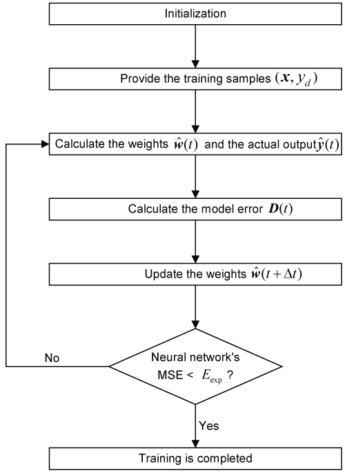
With the obtained D(t), we can execute the MPF iteration according to (17) and (19) to determine the weight matrix w. Figure 2 shows the procedure of the MPF-based weight optimization algorithm, which includes the following steps:

Step 1: Suppose the initial weights are small random numbers;

Step 2: Provide the training samples (x, y_d) for the network training, where x and y_d denote the input vector and target output value, respectively;

Step 3: Obtain the actual output $\widehat{y}(t)$ and model error D(t) by (17) and (19), respectively;

Step 4: Obtain the estimated weights $\widehat{w}(t+\Delta t)$ at t + Δt from the estimated weights $\widehat{w}(t)$ at time t and network model error D(t);

Step 5: Repeat the process from Step 2 to Step 4 if the mean square error (MSE) of the neural network is greater than the given tolerance E_exp. Otherwise, go to Step 6;

Step 6: End the iterative process of training. The weights resultant from Step (5) is optimal ones.

It can be seen from the above analysis, rather than minimizes the error function via gradient descent in BPNN, MPFNN uses an optimal estimation mechanism for weight optimization in the network training. Thus, it can effectively track measurement values via predicted information and estimated model error from the neural network. Further, unlike BPNN conducting the time-consuming line search at each iteration, MPFNN optimizes weights by compensating the disturbance of model error. Therefore, it can also avoid falling into local minimum and greatly reduce the training time.

Performance Evaluation and Discussions

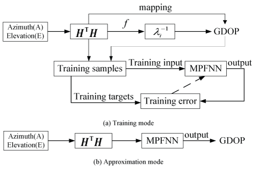
A prototype system has been implemented with the proposed MPFNN method for GDOP prediction. As shown in figure 3, there are two operation modes involved in MPFNN. When GPS signals are available, the network weights are updated by MPF in the training mode until the optimal network parameters are obtained. When satellite signals are blocked, i.e., GPS outages are occurred, MPFNN switches to the prediction mode to process the satellite information (E and A) from the remaining visible satellites on the input layer and predict GDOP values according to the latest weights obtained from available satellite signals.

Experiments and comparison analysis were conducted to evaluate the performance of the proposed MPFNN method for GDOP approximation. These experiments were conducted on an Intel Pentium IV 1.2 GHz and 2 G memory PC. The GDOP was computed every 1 min for 24 h and collected in two data samples with each of 720 samples. One data samples were used for the training purpose and the other for the approximation purpose.

Training performance

Trials were conducted to study the effect of the number of hidden neurons on the training performance of MPFNN. The hidden neurons are given by

$$N_{hid}=\{\begin{array}{l}\sqrt{N_{in}+N_{out}}+a\\ 2N_{in}+a\end{array}\left(20\right)$$

where N_in and N_out are the numbers of input and output layer neurons, and a is a random number between 0 and 10. According to (19) and (20), the number of hidden neurons falls into the ranges of (3, 13) and (20, 30).

5, 10, 20, 25 and 30 hidden neurons are selected to evaluate the training performance of MPFNN. MPFNN is initialized and trained with training samples. The network training process is conducted iteratively to minimize the error between the MPFNN output and desired response. The training process is terminated if the iteration number reaches 1000 or the minimized error is smaller than the given tolerance, which is set as the MSE of 10^-2. The time to update the weights in the training process is set as 60 s. The number of hidden layers of MPFNN is set as one.

For the comparison analysis, trials were conducted by both MPFNN and BPNN under the same conditions. Table 1 compares the training results of both methods under different numbers of hidden neurons. It can be seen from table 1 that the training accuracy is increased with the increase of hidden neuron number. For both methods, the MSE of 0.01 is not achieved within the entire test time in the case of 5 hidden neurons. This is because the number of hidden neurons is too small, leading to very limited training accuracy. For MPFNN, the MSE with 20 hidden neurons is much smaller than that with 5 hidden neurons, while the MSE with 25 hidden neurons is much smaller than that with 5 hidden neurons for BPNN.

However, the increase in the number of hidden neurons also leads to the increase of the training time. After the number of hidden neurons reaches a certain level, the improvement of accuracy is not significant. As shown in table 1, the training time of MPFNN for the case with 20 hidden neurons is the smallest. For the cases with 25 and 30 hidden neurons, the training time increases as the MPFNN architecture becomes more complex comparing to the case of 20 hidden neurons. However, the training accuracy is not improved significantly comparing to the case with 20 hidden neurons. Consequently, 20 hidden neurons provide the best training performance in terms of accuracy and computational time for MPFNN. Similarly, 20 hidden neurons is the most appropriate structure for BPNN.

The training accuracy of MPFNN is superior to that of BPNN under the same number of hidden neurons. Further, the iteration number and computational time of the MPFNN training are obviously smaller than those of the BPNN training under the same number of hidden neurons except for 5 hidden neurons.

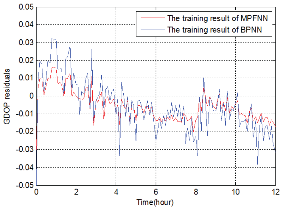
The GDOP residuals of both algorithms for the training case of 20 hidden neurons are illustrated in figure 4. It can be seen that the training accuracy of MPFNN is obviously superior to that of BPNN. The GDOP residuals generated by MPFNN are within (- 0.02, + 0.02), while within (- 0.04, + 0.04) for BPNN.

From the above, we can see that MPFNN outperforms BPNN in terms of training performance. The training time and error of BPNN is larger than those of MPFNN. This is mainly because BPNN suffers from the problem of local minimum, leading to the insufficient network learning process and hence limited accuracy. However, MPFNN is able to achieve higher prediction accuracy with much smaller training time, lead to the improved training performance comparing to BPNN.

Similar to BPNN, the proposed MPFNN method requires the selection of hidden neuron number. A small number of hidden neurons may lead to inadequate information to capture the characteristics of the desired response. A large the number of hidden neurons may cause an expensive computational load. The appropriate number of hidden neurons can be determined by conducting test computations to achieve the balance between the accuracy and computational load.

GDOP approximation

In this section, we shall compare the performances of MPFNN and BPNN in terms of GDOP approximation, both under an optimal structure. Based on the above analysis, the case of 20 hidden neurons provides the best outcomes for both MPFNN and BPNN. Therefore, it is chosen as the optimal structure for both methods.

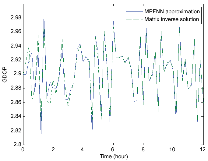
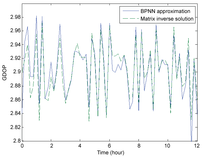
The GDOP approximation results of both MPFNN and BPNN are illustrated in figure 5 and figure 6, respectively, where the true values are obtained via MIS. It can be seen that after 4.7 hours the approximation curve of MPFNN is very close to the true values with the maximum deviation of 0.01, while the maximum deviation of 0.04 is remained in the approximation curve of BPNN.

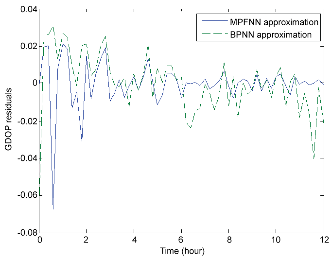
Figure 7 shows the GDOP approximation residuals of both methods, where the GDOP residual is defined as the difference between the actual output (by approximation) and target output (by matrix inversion). As shown in figure 7, although BPNN significantly decreases the oscillations, pronounced oscillations are still remained in the approximation curve during the entire test time. After four hours, the achieved GDOP residual by MPFNN is within (- 0.01, + 0.01), while within (- 0.04, + 0.02) by BPNN. Thus, it is evident that MPFNN has much higher accuracy than BPNN.

From the above, we can see that MPFNN has much higher accuracy for GDOP approximation than BPNN. This is because MPFNN uses MPF to optimize the neural network weights, where MPF corrects the neural network model error by compensating the deviation between the actual output and target output, and subsequently optimize the weights based on the corrected neural network model.

Acknowledgement

The work of this paper is supported by the Australian Research Council (ARC) Discovery Early Career Award (DECRA) (DE130100274).

Conclusions

This paper presents a new MPF-based neural network method for GDOP approximation. It adopts MPF in the neural network training process to optimize the neural network weights, leading to increased accuracy and reduced training time. The proposed method compensates the disturbance of the network model error by correcting the residual between the neural network's actual output and target output. It overcomes the BPNN problems such as local minimum and expensive training time. Experimental results and comparison analysis demonstrate that the proposed method outperforms BPNN for GDOP approximation.

Future research work will focus on the extension of the proposed MPFNN method from single-output to multiple-output of neural network structure. Algorithms will be developed to enable MPF to accept multiple outputs, thus establishing a MPF-based multi-output neural network for GDOP approximation.

References

1. A Noureldin, A EI-Shafie, M Bayoumi (2011) GPS/INS integration utilizing dynamic neural networks for vehicular navigation. Information Fusion 12: 48-57.
2. M Mosavi (2011) Applying genetic algorithm to fast and precise selection of GPS satellites. Asian Journal of Applied Sciences 4: 229-237.
3. H Azami, S Sanei, H Alizadeh (2012) GPS GDOP classification via advanced neural network training. The Third International Conference on Contemporary Issues in Computer and Information Sciences 29-31.
4. M Mosavi, M Azad, I EmamGholipour (2013) Position estimation in single-frequency GPS receivers using Kalman filter with pseudo-range and carrier phase measurements. Wireless Personal Communications 72: 2563-2576.
5. D Jwo, K Chin (2002) Applying back-propagation neural networks to GDOP approximation. The Journal of Navigation 55: 97-108.
6. S Doong (2009) A closed-form formula for GPS GDOP computation. Journal of GPS solutions 13: 183-190.
7. M Hamid, K Nitin (2013) Cascading artificial neural networks optimized by genetic algorithm and integrated with global navigation satellite system to offer accurate ubiquitous in urban environment. Computers, Environment and Urban Systems 37: 35-44.
8. W Jia, D Zhao, S Tian, et al. (2015) An optimized classification algorithm by BP neural network based on PLS and HCA. Applied Intelligence 43: 176-191.
9. X Chen, C Shen, W Zhang, et al. (2013) Novel hybrid of strong tracking Kalman filter and wavelet neural network for GPS/INS during GPS outages. Measurement 46: 3847-3854.
10. D Jwo, C Lai (2007) Neural network-based GPS GDOP approximation and classification. GPS Solution 11: 51-60.
11. D Simon, H El-Sherief (1995) Navigation satellite selection using neural networks. Neurocomputing, 7: 247-258.
12. S Tafazoli, M Mosavi (2011) Performance improvement of GPS GDOP approximation using recurrent wavelet neural network. Journal of Geographic Information System 3: 318-322.
13. H Azami, S Sanei (2014) GPS GDOP classification via improved neural network trainings and principal component analysis. International Journal of Electronics 101: 1300-1313.
14. A Tabatabaei, M Mosavi (2014) Rapid and precise GLONASS GDOP approximation using neural networks. Wireless Personal Communications 77: 2675-2685.
15. X Li, M Wu, X He, et al. (2013) The training method of general regression neural network for GDOP approximation. Applied Mechanics and Materials 278-280: 1265-1270.
16. H Azami, M Mosavi, S Sanei (2013) Classification of GPS satellite using improved back propagation training algorithms. Wireless Personal Communications 71: 789-803.
17. J Crassidis, F Markley (1997) Predictive filtering for nonlinear systems. Journal of Guidance Control and Dynamics 20: 566-572.
18. J Fang, X Gong (2010) Predictive Iterated Kalman Filter for INS/GPS Integration and Its Application to SAR Motion Compensation. IEEE Transactions on Instrumentation and Measurement 59: 909-915.
19. Y Zhao, S Gao, J Zhang, et al. (2014) Robust Predictive Augmented Unscented Kalman Filter. International Journal of Control, Automation and Systems 12: 996-1004.
20. VZ Marmarelis (2004) Appendix II: Gaussian White Noise, in Nonlinear Dynamic Modeling of Physiological Systems, John Wiley & Sons, Inc., Hoboken, NJ, USA. (doi: 10.1002/9780471679370.app2).
21. FL Lewis (1986) Optimal Estimation: With an Introduction to Stochastic Control Theory, New York: Wiley.