Journal of Petrochemical Engineering

Quantitative Determination of the Mineralogy from Elemental Logs by using the Particle Swarm Optimization Algorithm

Abstract

The purpose of this paper is to demonstrate the application of particle swarm optimization (PSO) algorithm for quantitative determination of mineral composition from the elemental logs in complex reservoirs. The mineralogy is necessary for the petrophysical and geological evaluation of the complex or unconventional reservoirs. Some common chemical elements in reservoir can be detected by the modern Geochemical logging technologies, and elemental weight fraction can obtained. The accurate conversion of elemental weight fraction to mineral content is the key and foundation for the subsequent applications in oil & gas exploration and development.

Keywords

Mineral content, Element weight fraction, Particle swarm optimization, Complex reservoir

Introduction

Minerals are the basic skeletons of rocks, and the mineralogy determines rock’s physical and chemical properties. The essential reservoir properties like porosity, permeability, and fluid saturations based on the mineralogy are very important in oil and gas exploration and development. The chemical properties of a reservoir rock are especially important in drilling, producing completing operations. The knowledge of mineralogy also provides information about the deposition and diagenesis of reservoir rocks which further helps in understanding flow characteristics in a reservoir. Mineralogy features directly leads to the difference in physical properties and consequently exert impacts on the reservoir performance in complex reservoirs lithologically. Mineralogy also impacts reservoir quality (RQ) and completion quality (CQ), which ultimately governs well performance and reservoir production [1]. The influence of mineral composition, characteristics and content on reservoir quality is the key problem that is required to be studied in depth.

In last decades the development and application of the geochemical log techniques has made possible to quantitative determination of the minerals along the drilling well. It is quite challenge to how accurate to determine the mineral composition from the elemental logs measured by the geochemical logging tool. This paper presents a methodology on quantitative determination of mineral from elemental logs by using the particle swarm optimization algorithm and its application in the complex reservoirs. This method takes into consideration the uncertainty of the element measurements and log response parameters. The theoretical response equation is based on the based on the mineral model of the reservoir and chemical formula of the minerals. The reconstructed element log curves were used to control the reliability of mineral analysis results.

Chemical Elements Detected in Reservoir

With recent advances in logging technology (geochemical log or elemental log), it is able to generate a comprehensive, continuous measurement of major chemical elements in the subsurface [2]. The major chemical elements in the formation are currently measured by the spectroscopy logging tool from the GST, ECS, Litho Scanner GEM, FleX, EMT and FEM with the gamma ray capture and inelastic spectrum processing as well as the X-ray fluorescence technology. Table 1 shows the major elements detected and the detecting/processing methods.

Rock & Mineral Volumetric Model and Log Responses

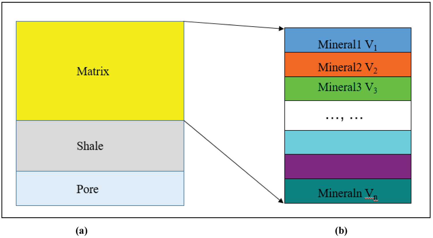
Actually any reservoir rock can be described by using the following volumetric model, which is consisted of the matrix, shale and pore (fluids), and the matrix is consisted of the lots of the minerals. Figure 1 shows a sketch of the reservoir rock and the rock matrix.

Based on the measuring principle of the geochemical log tool, the log response of the reservoir rock can be written as follows in theory,

$$\log ={\log }_{ma}\ast V_{ma}+{\log }_{sh}\ast V_{sh}+{\log }_f\ast \varnothing$$

The log response of the matrix can be determined by the following equation,

$${\log }_{ma}=\frac{\log -{\log }_{sh}\ast V_{sh}-{\log }_f\ast \varnothing }{1-V_{sh}-\varnothing }$$

Where, the log denotes log response of the reservoir; the log _ma , log _sh and log _f denote the log response of the rock matrix, the shale the pore fluids in reservoir respectively; the V _ma (= 1 – V _sh – Ø), V _sh and Ø denote the volumetric content of the rock matrix and the shale as well as the porosity in reservoir.

Based on the above mineral volumetric model in Figure 2, the log response of the rock matrix can be written as follows,

$${\log }_{ma}={\log }_1\ast V_1+{\log }_2\ast V_2+\cdot \cdot \cdot +{\log }_n\ast V_n$$

For rock matrix which is consisted of the ( i = 1, 2, ..., n ) minerals, the log response equation of the density and volumetric photoelectric factor is as following,

$${\rho }_{ma}={\rho }_1{V}_1+{\rho }_2{V}_2+\cdot \cdot \cdot ,\mathrm{...}+{\rho }_n{V}_n$$

$$U_{ma}=U_1{V}_1+U_2{V}_2+\cdot \cdot \cdot ,\mathrm{...}+U_n{V}_n$$

The log response equation for any element weight fraction is,

$$EL=C{o}_1\frac{{\rho }_1}{{\rho }_{ma}}{V}_1+C{o}_2\frac{{\rho }_2}{{\rho }_{ma}}{V}_1+\cdot \cdot \cdot ,\mathrm{...}+C_n\frac{{\rho }_n}{{\rho }_{ma}}{V}_n$$

Combining the above log responses, the general format of log response for the mineral quantitative determination is

$$f_j\left(V\right)={\displaystyle \sum _{i=1}^n{C}_{ji}\ast V_i}$$

Where, the ρ _ma , U _ma and EL denote respectively the density, photoelectric factor and element weight fraction which are from geochemical log; the V (= V ₁ ,V ₂ ,…,V _n ) denotes the mineral volumetric content; the ρ (= ρ ₁ , ρ ₂ , …, ρ _n ) log response of the mineral for density log; the U (= U ₁ , U ₂ , …, U _n ) denotes the log response of the mineral for volumetric photoelectric factor log; the Co (= Co ₁ , Co ₂ , …, Co _n ) denotes the ratio between the element atomic mass and the mineral molecular mass; the C _ji denotes the j ^th log response parameter of the i ^th mineral.

Principle of Particle Swarm Optimization (PSO)

Particle swarm optimization is a heuristic global optimization method put forward originally by Doctor Kennedy and Eberhart in 1995 [3]. It is developed from swarm intelligence and is based on the research of bird and fish flock movement behavior. In the PSO algorithm, a point in the search space (i.e., a possible solution) is called a particle. The collection of particles in a given iteration is referred to as the swarm. In the basic particle swarm optimization algorithm, particle swarm consists of “M” particles, and the position of each particle stands for the potential solution in N-dimensional space. Each particle's movement is influenced by its local best known position, but is also guided toward the best known positions in the search-space, which are updated as better positions are found by other particles. This is expected to move the swarm toward the best solutions.

Assume there is a particle swarm X = {X ₁ , X ₂ , …, X _M } formed by the M particles in a N-dimensional search space. The particles change its condition according to the following three principles: (1) To keep its inertia; (2) To change the condition according to its most optimist position; (3) To change the condition according to the swarm’s most optimist position. Assuming the position and the speed of the i ^th particle at time “t” are represented as X _i = (x _i1 , x _i2 ,…, x _in ) and V _i = (v _i1 , v _i2 , …, v _in ) respectively. P _i ^L = (p _i1 , p _i2 , …, p _in ) denotes the best position which the i ^th particle has achieved so far, and P _g = (p _g1 , p _g2 , …, p _gn ) is the best of p _i (t) for any I = 1, 2, …,... N. At each iteration, each particle in the swarm moves to a new position in the search space. We denote x as a potential solution in the search space of a N-dimensional optimization problem, X _i (t) = (x _i1 , x _i2 ,...,x _in ) as the position of the i ^th particle in iteration “t”. Each iteration process of the particle velocity and position are given as follows,

$$V_i(t+1)=w{V}_i(t)+c_1{r}_1(P_i^L-X_i(t))+c_2{r}_2(P_g-X_i(t))$$

$$X_i(t+1)=X_i(t)+V_i(t+1)$$

Where c ₁ and c ₂ are the learning factors, usually they are the constants in the interval (0, 2). r ₁ and r ₂ are the random numbers in the interval (0, 1). V _i (t) denotes the velocity of the i ^th particle at time “ t ”, the updated value of which needs to be determined by the value of previous time, i.e., the particles maintain a velocity inertia. w (€ = (0, 1)) denotes the inertia weight, which controls the search space capabilities of particles, the greater the value, the greater the search space scope of particles.

Optimization Objective Function and Mineral Quantitative Determination

With the elemental log curves (Si, Fa, Al, Fe, Mg, et al.) as well as density and photoelectric factor curves from geochemical log, a workflow of the mineral content analysis is shown in the Figure 2. This is an iterating procedure by 1) Optimizing the objective function and obtaining the mineral content; 2) Reconstructing the corresponding element log curves and controlling the results; 3) Modifying the mineral model and parameters; and 4) Optimizing the objective function and obtaining the mineral content again.

When the mineral volumetric model is determined for a certain reservoir, the objective fitness function which is based on the above log response equations can be written as follows,

$$\min \Delta =\sqrt{\frac{1}{m}}{\displaystyle \sum _{j=1}^m\frac{{\left(f_j\left(V\right)-L_j\right)}^2}{{\sigma }_j^2+{\tau }_j^2}}$$

With the constraints are as following,

1) ${\displaystyle \sum _{i=1}^n{V}_i}=1.0$

2) $V_i\le 1.0$ i = 1, 2,…,.. n

3) $V_i\ge 0.0$ i = 1, 2,…,…n

where, V is the mineral content will be obtained, the subscript i ( =1,2,..,…n ) is the i ^th mineral; f _j ( V ) is the j ^th theoretical log response, the L _j is the j ^th measuring log curve which includes the density, photoelectric factor and the element weight fractions in Table 1, the subscript j ( =1,2 , …,… m ) is the number of the available log curve; σ _j is the uncertainty bias of the j ^th theoretical log response, τ _j is the uncertainty bias of the j ^th measuring log curve.

It is quantitatively determined for the mineral content in a certain complex reservoir by using the particle swarm optimization to optimize above objective function with constraints, based on the mineral model (Figure 1), chemical formula and the log response parameters of mineral shown in the Table 1 and Table 2.

Applications

The above methodology is applied to carry out the analysis and processing of the element loggings and to quantitatively determine the mineral content in the lithological complex reservoirs. The three case studies are presented in this paper, one is in a carbonate reservoir and the elements were detected by the ECS tool with the inelastic gamma ray spectrum; the second is in an igneous reservoir and the elements were detected by the ECS tool with the capture gamma ray spectrum; the third is in a carbonate reservoir and elements were detected by the EMT tool with the capture gamma ray spectrum.

Case Study 1

This is one well in a carbonate formation, which the elements detected by ECS tool with the inelastic gamma ray spectrum. The major detected elements are Ca, Si, Mg, Al, Fe and others (Gd, K, Mn, Na, Su and Ti) are minor in this carbonate formation. With the above 5 major elemental logs as well as the matrix density and volumetric photoelectric factor, a certain fitness objective function, which is 7 log curves and 6 mineral contents, is established and used to optimizing process. The mineral contents of the Calcite, Dolomite, Quartz, Ankerite, Anhydrite and Siderite are determined quantitatively. Figure 3 presents the result of the mineral analysis for this case study. In the Figure 3 track 1 shows gamma ray curve; track 2 shows Sulfur (DWSU), Silicon (DWSI) and Aluminum (DWAL) weight fraction; track 3 shows Magnesium (DWMG), Calcium (DWCA) and Iron (DWFE) weight fraction; track 4 shows the density and volumetric photoelectric factor of matrix; track 5 shows the mineral (Quartz, Calcite, Dolomite, Anhydrite, Ankerite and Siderite) volumetric contents determined. It shows a very consistent between the elemental fraction and mineral content.

Figure 4 presents the quality control of the mineral analysis. In the Figure 4, track 1 shows the mineral content; track 2 shows the measured density (RHOZ) and volumetric photoelectric factor (UMA) as well as the reconstructed density (RHOMA2) and volumetric photoelectric factor (UMA2) from the mineral contents; track 3 shows the measured Silicon (DWSI) and Calcium (DWCA) content as well as the calculated Silicon (SI2) and Calcium (CA2) contents; track 4 shows the measured Iron (DWFE) and Sulfur (DWSU) contents as well as the reconstructed Iron (FE2) and Sulfur (SU2) contents; track 5 shows the measured (DWMG) and the reconstructed (MG2) Magnesium contents. The quality control of the mineral analysis from element logs can carried out by comparing the measured and calculated element and density curves. In this case QC shows a not good matching for Iron element content curve in whole well and not good matching for the Magnesium content curve in the shale zones. This is as the clay mineral is not inputted into the mineral model and objective function in this carbonate formation, which includes the Iron and Magnesium element, but unknown clay mineral type (Chlorite or Illite) and their chemical formula. So that for this case mineral results in the reservoir zone are confidence, the uncertainty of mineral results exists in the shale zones.

Case Study 2

This is one well in an igneous formation, which the elements detected by ECS tool with the capture gamma ray spectrum. The major detected elements are the Ca, Si, Al, Fe and the others (Cl, Gd, H, Su and Ti) are minor in this igneous formation, With the above 4 major elemental logs as well as the matrix density and volumetric photoelectric factor, a certain fitness objective function, which is 6 log curves and 4 mineral contents, is established and used to optimizing process. The mineral contents of the Quartz, Albite, Anorthite and Augite are determined quantitatively. Figure 5 presents the result of the mineral analysis for this case study. In the Figure 5 track 1 shows gamma ray curve; track 2 shows Sulfur (DWSU), Silicon (DWSI) and Aluminum (DWAL) weight fraction; track 3 shows Calcium (DWCA) and Iron (DWFE) weight fraction; track 4 shows the density and volumetric photoelectric factor of matrix; track 5 shows the mineral (Quartz, Albite and Anorthite, Augite) volumetric contents determined. It shows a very consistent between the elemental fraction and mineral content.

Figure 6 presents the quality control of the mineral analysis. In the Figure 6, track 1 shows the mineral content; track 2 shows the measured density (RHOZ) and volumetric photoelectric factor (UMA) as well as the reconstructed density (RHOMA2) and volumetric photoelectric factor (UMA2) from the mineral contents; track 3 shows the measured Silicon (DWSI) and Calcium (DWCA) contents as well as the reconstructed Silicon (SI2) and Calcium (CA2) contents; track 4 shows the measured Iron (DWFE) and the reconstructed Iron (FE2) content; track 5 shows the measured (DWAL) and the reconstructed (AL2) Aluminum contents. The quality control of the mineral analysis from element logs can carried out by comparing the measured and calculated element and density curves. In this case it shows very confidence for the mineral analysis result as the very good matching is obtained between the measured and reconstructed curves in the whole well.

Case Study 3

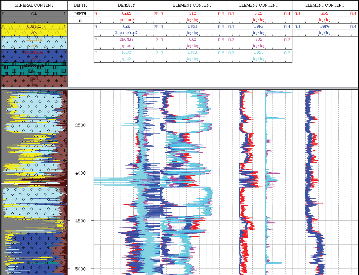
This is one well in a carbonate formation, which the elements detected by EMT tool with the capture gamma ray spectrum. The major detected elements are the Ca, Si, Mg, Al, Fe, Sand others (Gd, Mn, K and Ti) are minor in this carbonate reservoir. With the above 6 major elemental logs as well as the matrix density and volumetric photoelectric factor, a certain fitness objective function, which is 8 log curves and 6 mineral contents, is established and used to optimizing process. The mineral contents of the Calcite, Dolomite, Quartz, Anhydrite, Pyrite and Kaolinite are determined quantitatively in this carbonate formation. Figure 3 presents the result of the mineral analysis for this case study. In the Figure 7 track 1 shows gamma ray curve; track 2 shows Sulfur (DWSU), Silicon (DESI) and Aluminum (DWAL) weight fraction; track 3 shows Magnesium (DWMG), Calcium (DWCA) and Iron (DWFE) weight fraction; track 4 shows the density and volumetric photoelectric factor of matrix; track 5 shows the mineral (Kaolinite, Quartz, Calcite, Dolomite, Anhydrite and Pyrite) volumetric contents determined. It shows a very consistent between the elemental fraction and mineral content.

Figure 8 presents the quality control of the mineral analysis. In the Figure 8, track 1 shows the mineral content; track 2 shows the measured density (RHOZ) and volumetric photoelectric factor (UMA) as well as the reconstructed density (RHOMA2) and volumetric photoelectric factor (UMA2) from the mineral contents; track 3 shows the measured Silicon (DWSI) and Calcium (DWCA) content as well as the reconstructed Silicon (SI2) and Calcium (CA2); track 4 show the measured Iron (DWFE) and Sulfur (DWSU) curves as well as the reconstructed Iron (FE2) and Sulfur (SU2) content curves; track 5 shows the measured Magnesium (DWMG) and Aluminum (DWAL) curves and the reconstructed Magnesium (MG2) and Aluminum (AL2) content curves. The quality control of the mineral analysis from element logs can carried out by comparing the measured and reconstructed log curves. There is a very good fitness between the measured and reconstructed curves in the reservoir zone. It shows the confidence for the mineral analysis. In the shale there is an uncertainty for the mineral analysis result as there are some difference between the he measured and reconstructed curves [4-12].

Conclusion

With the element logs detected by geochemical log tool, mineral composition can be quantitatively determined by using a powerful intelligent technique (PSO). In the reservoir zone the mineral analysis results are more confidence as the physical and chemical property are stable. In the shale the clay mineral analysis results are with some uncertainty as the physical and chemical property are variable. By using the methodology mention in this paper, it will be also give the very confidential mineral analysis results when the mineral type and properties are well known. Understanding the geology background is also very important to quantitatively determine the mineral content from the element logs.

References

1. Diaz HG, Miller C, Lewis R, et al. (2013) Evaluating the impact of mineralogy on reservoir quality and completion quality of organic shale plays. AAPG Rocky Mountain Section Meeting, 22-24.
2. Mac Donald RM, Bradford CM, Meridji Y, et al. (2011) Comparison of elemental and mineral abundances from core and three modern neutron induced elemental spectroscopy tools. SPWLA 52nd Annual Logging Symposium. SPWLA-2011-BBB.
3. Kennedy J, Eberhart R (1995) Particle swarm optimization. Proc of IEEE International Conference on Neural Network 1995: 1942-1948.
4. Modares H, Alfi A, Naghibi-Sistani M-B, et al. (2010) Parameter estimation of bilinear systems based on an adaptive particle swarm optimization. Engineering Applications of Artificial Intelligence 23: 1105-1111.
5. Rao RV, Patel VK (2010) Thermodynamic optimization of cross flow plate-fin heat exchanger using a particle swarm optimization algorithm. International Journal of Thermal Sciences 49: 1712-1721.
6. Shehata RH, Mekhamer SF, El-Sherif Nehad, et al. (2014) Particle swarm optimization: Developments and application fields. International Journal on Power Engineering and Energy (IJPEE). 5.
7. Shi Y, Eberhart RC (1998) A modified particle swam optimizer. IEEE Word Congress on Computational Intelligence, Anchorage.
8. Li W, Shanshan W, Wei Y, et al. (2011) Improved method of particle swarm impedance inversion and its application. J Lithologic Reservoirs 23: 103-106.
9. Zhang Y, Salisch HA (1998) Study and applications of ‘model-optimization’- A log evaluation method to determine permeability in lithologically complex formations. Geo-Triad’98. 15-19.
10. Yi-an C, Tong-xin J, Xi-yang L, et al. (2013) Inversion of multi-anomalies in resistivity profiling based on particle swarm optimization. Progress in Geophysics 28: 2164-2170.
11. Dai QW, Chen W, Zhang B, et al. (2019) Improved particle swarm optimization and its application to full-waveform inversion of GPR. Geophysical and Geochemical Exploration 43: 90-99.
12. El-Shorbagy MA, Hassanien AE, (2018) Particle swarm optimization from theory to applications. International Journal of Rough Sets and Data Analysis. 5.