Fully Coupled Thermo-Mechanical Modelling of the Initial Phase of the Friction Stir Welding Process Using Finite Element Analysis

Abstract

In the present study a finite element model of the FSW process is built and a FSW but weld of two aluminium alloy 2024-T3 plates is simulated using a fully coupled thermo-mechanical analysis. Besides the welded panels, the model includes the backing plate and the welding tool as physical bodies, which makes the simulations more realistic. The model also includes conductive heat transfer between the contact surfaces of the FSW tool, the aluminium plates and the backing plates, heat generation due to friction between the tool and the welded plates and heat loss to the ambient air due to convection.

The simulated model makes it possible to analyse and check several aspects of this welding technique. It is proved that tool geometry has a vital importance in the FSW process. The influence of using instantaneous or ramped velocity at the beginning of the simulations is also studied. Moreover, it is seen that the mesh used in the finite element analysis and the adjustment of the inelastic heat fraction have a great influence on the obtained results.

Introduction

Friction Stir Welding (FSW) is a relatively new developed solid state joining technique. FSW process was invented by Wayne Thomas at The Welding Institute (TWI) in December 1991 [1], and since its invention, it has shown to be viable for joining many kinds of materials of various thicknesses, including hard-to-weld materials like aluminium alloys, magnesium, stainless steel, copper alloys, zinc and titanium alloys. Due to this large range of materials and thicknesses, FSW technique has been successfully applied to a lot of fields, such as aerospace, ship and automobile industries. Now days there are lots of opened investigations to develop the design and the materials of the FSW tools in order to enable more materials to be welded by using this process. An important difficulty is to find tool materials capable of operating at the forging temperatures of the work pieces.

The main feature of FSW is that the weld takes place in a solid phase below the melting point of the material to be joined, which permits to preserve better the mechanical properties of these materials and reduce the deformation due to thermal expansion [1]. In addition to these advantages, compared with the traditional welding techniques, FSW is energy efficient and environment friendly [2].

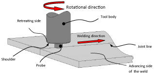
In FSW method, a rotating tool in contact with the work pieces causes the necessary frictional heating and the mechanical deformation for the welds. The rotating tool is inserted into the butt of the welding plates. With the rotation this tool, the material close to the tool-plate interface becomes thermo-plastic, and then, a joint can be formed by adding a translational movement to the rotation of the welding tool. The tool consists of a cylindrical body where a probe is attached on the bottom surface. This probe, also known as pin, is the part of the tool which is inserted into the joint line between the two plates that are to be welded. Even though friction between the pin and the plates helps to increase the temperature of the work pieces, the vast majority of the total frictional heating is generated at the bottom surface of the tool, which is known as shoulder.

The shoulder is responsible for major heat contribution. Hence, to improve the joint properties and minimizing the defects the concept of shoulder designs emerged. The plane, concave and convex shoulder designs were widely adopted tool designs for which considerable research was carried out by many researchers. The systematic review conducted by [3] on FSW tools, takes a new look in tool design based on various aspects, one of which was the nature of shoulder surface at the tool/material interface. They also presented various possible shoulder end designs and discussed the use of one such design that is scrolled shoulder which facilitates the material flow from the edge of the shoulder to the pin [4] studied various shoulder geometric effects on 1 mm thick copper sheets and observed that scrolled shoulder geometry has more effective material flow.

Several authors among others have studied the tool pin influence on the mechanical properties of the weld. The study conducted by [5] on the effect of tool geometry revealed that the geometry of the pin plays a key role only in the material deformation and moreover the heat generation developed by the pin was relatively insignificant to the weld [6] investigated with copper friction stir welds using and threaded and square tool pin and found that due to the eccentricity action of the edges, the tool pin with square resulted in finer grains thus lead to superior properties compared to conical tool pin profile. The investigation of [7] during the friction stir welding of Al 6063 alloys with different tool pins showed that the tapered circular and polygonal pins result in defects compared to square tool pin. The welds with square tool pin profile achieved superior mechanical properties compared to other tool pin. The attempts by [8], to study the adhesion of plasticized material in polygonal tool pin profiles showed that at higher weld pitch (traverse speed up on rotational speed) the pins with less number of sides avoids permanent adhesion and the stresses were observed to be low for pins with larger number of sides. They developed a relation for obtaining the optimum sides of the polygon pin for a given set of FSW conditions and it was related to the weld pitch. In a similar attempt, [9] used the polygonal tool pins which have the capability to improve the mechanical strength of the joint compared to circular pin tools and analyzed the sticking torque experienced by the polygonal pins along with the rate of heat generation.

FSW process is characterized by large deformation and higher strain rates, making Finite Element modelling of the process highly complex. In addition to the experimental studies, many numerical studies have been performed to increase the understanding of different aspects of the FSW process [10] presented a three-dimensional sequentially coupled thermo-mechanical analysis of the friction stir welding process suitable for residual stress prediction [11] presented a three-dimensional continuum based finite element model for the FSW process. The model is thermo-mechanically coupled with rigid-viscoplastic material behavior and the simulation was used to investigate the temperature and strain in the heat affected zone [12] investigated the material flow patterns in FSW welds of the aluminum alloy 6061-T6 under varying welding conditions [13] studied the material flow in FSW welds of 1018 steel under different process parameters using a finite element model with rate-dependent material behavior [14] have simulated three dimensional coupled thermo-mechanical analysis using Lagrangian implicit code in DEFORM-3D. They have simulated plunging and welding stages by defining work piece as a rigid viscoplastic material.

Some of the recent works are among others are [15-18]. [15] developed a meshless particle method for the analysis of transient heat transfer during FSW process. The heat source model is based on sticking friction and it was used to describe the heat generation [16] proposed a three dimensional coupled thermo-mechanical finite element to simulate a FSW process based on Lagrangian incremental technique with a work piece considered as a rigid viscoplastic material [17] proposed a numerical procedure, based on a finite element approach, is proposed to simulate multiple three-dimensional crack propagation in a welded structure [18] a rate-dependent Johnson-Cook constitutive model was used to capture elastoplastic work deformations during FSW.

When the top surface of the plates establishes contact with the rotating shoulder surface, the temperature increases and it softens the material up and enables the probe to traverse the joint line and stir the material in order to make the weld. The remaining fraction of the heat is generated due to the high rate plastic deformation of the weld material next to the probe. Figure 1 illustrates the FSW process.

One of the most important factors in the FSW processes is the tool technology. It was early realized that an accurate design of the welding tool was essential in achieving joints with good mechanical properties. The tool design has two main aspects. The first one is to find a tool material that has to be able to work at the forging temperatures of the weld materials. The other aspect is the tool geometry. A concave shoulder profile helps the material displaced by the probe to remain under the shoulder area. It also makes possible to maintain the pressure in order to obtain a good welding. As regards the probe, threaded probes has shown to improve the drilling of the thicker plates. Besides, lots of probe geometries have been developed to get better material flow around the tool, such as conical, oval and paddle shapes. It is also important to have a radius to smooth the change in section between the shoulder and the probe in order to reduce stress concentrations.

Besides the tool material and geometry, other parameters have an important role during the FSW process and determine the quality of the welded joints. These main parameters are the plunge depth, the tool tilt angle, the rotational speed and the traverse speed. The plunge depth is defined as the depth of the lowest point of the shoulder below the top surface of the weld pieces. The pressure below the tool is increased by plunging the shoulder below the top surface of the plates, and it helps to ensure a good forging behind the tool. Thus this parameter needs to be correctly set, because the pressure under the tool can be reduced by a too short plunge depth, which may result in flaws in the weld. On the other hand, setting too much plunge depth can damage the backing plate surface. Tilting the tool by a few degrees, with the result that the front of the tool is higher than the rear, also improves the welding quality. As it has been said before, there are two tool seeds to be considered in FSW, the rotational speed and the traverse speed. In general, it has been shown that increasing the rotational speed or decreasing the traverse speed will lead to a hotter weld. The material surrounding the tool has to be hot enough in order to enable the plastic flow required and minimise the forces acting on the tool. Voids and other flaws can appear in the stir zone if the material is too cool, and even the tool may break. Thus heat input should be sufficiently high to guarantee suitable material plasticity, but not so high that the mechanical properties of the welded material are excessively affected.

The present study takes a previous model of FSW [10] as the starting point and develops it. An experimental weld [19] is used as a guideline to build the finite element (FE) model of FSW. This experimental weld is a 105 mm friction stir butt weld of two plates made of the aluminium alloy 2024 T3 (AA2024-T3). The FSW process is simulated using the finite element software ABAQUS [20]. The paper focuses on the initiation of the FSW process i.e. the plunge, dwell, initiation of the rotational velocity. Although this initial phase has limited effect on the quality of the weld itself it is an important step in the numerical procedure towards modelling the complete process.

Theoretical Background

The final results are obtained solving these thermal and mechanical equations by use of finite element analysis. Appropriate boundary conditions are applied in the analysis. The thermal equilibrium equation for the energy balance of the model is the three-dimensional advection-diffusion equation

$$\rho \cdot c_p\cdot \left(\frac{\partial \theta }{\partial t}+\nabla \theta \cdot v\right)-\nabla \cdot \left(k\cdot \nabla \theta \right)-q=0(2.1)$$

Where $\theta \left(r,t\right)$ is the temperature at a point r and at a time t, ρ is the mass density, C_p is the specific heat, v is the velocity vector of the advective flow, k is the thermal conductivity matrix and q is the possible body heat flux added from external and internal sources. The gradient operator, ∇(θ) is defined as vector field whose components are the partial derivatives of θ with respect to the spatial coordinates.

The solution for the displacements, deformation, stresses, forces, and other state variables requires that, both force and moment equilibrium should be conserved over any arbitrary volume of the body, which is analysed. The exact equilibrium statement is presented below.

Considering that V is a volume occupied by a part of the body in the current configuration, and S is the surface bounding this volume, the force equilibrium equations are given by

$${\displaystyle \underset{S}{\int }tdS}+{\displaystyle \underset{V}{\int }fdV}=0(2.2)$$

Where t is the surface traction vector at any point on S, i.e. force per unit of current area, and f the body force vector at any point within the volume V, i.e. force per unit of current volume. The Cauchy stress tensor σ at a point of S is defined by

$$t=n\cdot \sigma (2.3)$$

Where n is the unit outward normal vector to the surface S at the point. Using this definition, equation (2.2) is

$${\displaystyle \underset{S}{\int }n\cdot \sigma dS}+{\displaystyle \underset{V}{\int }fdV}=0(2.4)$$

Applying the Gauss theorem to the surface integral in the equilibrium equation and taking into account that the volume V is arbitrary, the local force equilibrium differential equations is given by

$$\nabla \cdot \sigma +f=0(2.5)$$

Moment equilibrium is most simply written in the general case by taking moments about the origin

$${\displaystyle \underset{S}{\int }\left(x\times t\right)dS}+{\displaystyle \underset{V}{\int }\left(x\times f\right)dV}=0(2.6)$$

Where x is the position vector. Use of the Gauss theorem with equations (2.5) and (2.6) then leads to the result that the Cauchy stress tensor must be symmetric:

$$\sigma ={\sigma }^T(2.7)$$

It should be noted that the moment equilibrium equation (2.6) assumes that there are no point couples acting on the volume. More detail about the week and strong formulation of the energy balance and balance of linear and angular momentums can be found in [21].

Constitutive relations

The material of the plates modelled in this study is modelled as a thermo elastic-plastic Von Mises material. On the one hand, the elastic properties of this material are assumed to be isotropic and linear with temperature dependent Young's modulus. On the other hand, the hardening of the material is modelled as temperature dependent linear kinematic hardening. Using the additive strain rate decomposition, the total strain rate ${\dot{\epsilon }}_{ij}$ can be written in terms of the elastic, plastic and thermal strain rates as

$${\dot{\epsilon }}_{ij}={\dot{\epsilon }}_{ij}^{th}+{\dot{\epsilon }}_{ij}^{el}+{\dot{\epsilon }}_{ij}^{pl}(2.8)$$

In this equation, the thermal strains are given by

$${\epsilon }_{ij}^{th}=\alpha \left(\theta -{\theta }_I\right){\delta }_{ij}(2.9)$$

where α is the thermal expansion coefficient, θ is the current temperature, θ_I(is the initial temperature and δ_ij is Kronecker's delta, which is defined by

$${\delta }_{ij}=\left\{\begin{array}{c}1ifi=j\\ 0ifi\ne j\end{array}\right\}(2.10)$$

Hooke's law defines the isotropic constitutive relation law for the elastic strains by

$${\epsilon }_{ij}^{el}=\frac{1+\nu }{E\left(\theta \right)}{\sigma }_{ij}-\frac{\nu }{E\left(\theta \right)}{\delta }_{ij}{\sigma }_{kk}(2.11)$$

Where v is Poisson's ratio, E(θ) is the temperature dependent Young's modulus.

Finally, the plastic behaviour is represented by a pressure-independent plasticity model. For this model the yield surface f, which bounds the elastic region, is defined by the function

$$f=\sqrt{\frac{3}{2}\left(s_{ij}-{\alpha }_{ij}\right)\left(s_{ij}-{\alpha }_{ij}\right)}-{\sigma }_{y0}\left(\theta \right)=0(2.12)$$

Where α_i,j is the backstress tensor, ${\sigma }_{y0}\left(\theta \right)$ is the temperature dependent yield stress at zero plastic strains and S_ij is the deviatoric stress tensor given by

$$s_{ij}={\sigma }_{ij}-\frac{{\sigma }_{kk}}{3}{\delta }_{ij}(2.13)$$

This model assumes associated plastic flow, which is represented by the function

$${\dot{\epsilon }}_{ij}^{pl}=\frac{\partial f}{\partial {\sigma }_{ij}}{\dot{\epsilon }}_{eff}^{pl}=\frac{\partial f}{\partial {\sigma }_{ij}}\sqrt{\frac{2}{3}{\dot{\epsilon }}_{kl}^{pl}{\dot{\epsilon }}_{kl}^{pl}}(2.14)$$

As it was said above, this study uses the linear kinematic hardening model. In this model, the evolution of the backstress tensor σ_ij is defined by Ziegler's hardening rule, generalized to the non-isothermal case as

$${\dot{\alpha }}_{ij}=C\left(\theta \right){\dot{\epsilon }}_{eff}^{pl}\frac{1}{{\sigma }_{y0}\left(\theta \right)}\left({\sigma }_{ij}-{\alpha }_{ij}\right)+\frac{1}{C\left(\theta \right)}{\alpha }_{ij}\dot{C}(2.15)$$

Where C(θ) is the hardening parameter, given by the slope of the isothermal uniaxial stress-strain response, $d\sigma /d{\epsilon }_{}^{pl}$, taken at different temperatures.

FE-Model Description

Parts

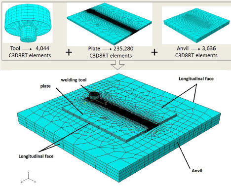
The model consists of three parts or pieces, which are the plate, the tool and the anvil. It is worth mentioning that there is only one plate of 150 × 120 × 5.85 mm. This result from simulating the two plates of 150 × 60 × 5.85 mm are modelled as one, representing that they are held together by the clamps. The unique plate is modelled as a three-dimensional deformable body and the material assigned to it is aluminium alloy 2024-T3, which is defined below. 235,280 8-node linear brick elements C3D8RT form the mesh of the work pieces, which is finer at the weld zone in order to improve the accuracy of the results. These elements are designed for coupled thermo-mechanical analyses and include reduced integration and hourglass control.

A three-dimensional revolved rigid body with the geometrical features explained in section 1.2 models the welding tool. Steel AISI H13 is assigned as the tool material. Using a rigid body condition allows having a non-deformable tool without losing its thermal properties, and reduces computational costs at the same time. Element type used to mesh the tool part is also C3D8RT, but the mesh is not as fine as the mesh of the weld zone of the plate, due to the application of rigid body condition. The mesh of the tool has 4,044 elements.

Finally, the anvil of 240 × 240 × 25 mm is a three-dimensional deformable body also meshed with 3,636 C3D8RT elements. This small number of elements results from the boundary conditions applied to the anvil and the plate, which simplify the model constraining the displacement of anvil nodes in all directions. Thus the anvil only dissipates heat from the plate without becoming deformed. Common medium carbon steel properties detailed below are assigned to the anvil part.

These three parts are assembled as illustrated in Figure 2. It should be noted that the tool tilt angle is neglected in the model.

Material properties

To simulate the FSW process, three different materials are used, one for the plate, one for the tool and another one for the anvil. The material properties and the material model of those three materials are detailed below.

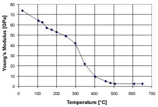
The plates are made of the aluminium alloy 2024-T3, thus the model for this material is the most complex of all three material models used here. The main interest in using this material in the FSW process is that its weld ability is poor using fusion weld techniques. During the simulations the material is modelled as an isotropic thermo-elastic-plastic Von Mises continuum with kinematic hardening. Concerning the AA2024-T3 properties, the temperature effect on mass density and Poisson's ratio is very modest. Thus both parameters are assumed to be constant and set to ρ = 2770 kg/m³ and ν = 0.33 respectively. The conductivity and the specific heat are set to k = 120 W/(m ℃) and cp = 875 J/(kg ℃) respectively [22]. Experimental data for the temperature effect on the thermal expansion coefficient, α, are fitted as a linear approximation and varies from 2.43.10-5 ℃^-1 to 2.8.10-5 ℃^-1 over the temperature range 20 ℃ to 500 ℃ [22]. Throughout the welding process, the temperature of the AA2024-T3 plates is varying from room temperature to temperatures near to the melting point of this material, which is 502 ℃. The mechanical properties, such as the yield stress and the elastic parameters, in particular the Young's modulus, are influenced by these changes. But the yield strength is not only temperature dependent, since the strong plastic deformation of the plates during the welding process and temperature history also affects it considerably [23]. Table 1 presents the stress-strain data used during the simulations, and Figure 3 shows the influence of the temperature on the Young's modulus.

The material model for the AA2024-T3 used during the fully coupled thermal-stress analysis also includes an inelastic heat fraction, η, which provides for inelastic energy dissipation as a heat source. Plastic straining gives rise to a heat flux per unit volume of $q^{pl}=\eta \sigma :{\dot{\epsilon }}^{pl}$ , where q^pl is the heat flux that is added into the thermal energy balance, η is the inelastic heat fraction set to 0.9 (assumed constant), σ is the stress, and ${\dot{\epsilon }}^{pl}$ is the rate of plastic straining [22]. The Johnson-Cook damage initiation criterion [22] and [24] is also included in the material model in order to predict the onset of damage due to nucleation, growth, and coalescence of voids in the material of the plates. In this criterion the equivalent plastic strain at the onset of damage, ${\epsilon }_f^{pl}$, is assumed to be of the form ${\epsilon }_f^{pl}=\left[d_1+d_2\exp \left(d_3\frac{p}{q_M}\right)\right]\left[1+d_4^{}\ln \left(\frac{{\dot{\epsilon }}^{pl}}{{\dot{\epsilon }}^0}\right)\right]\left(1+d_5\stackrel{⌢}{\theta }\right)$, where $d_1$ - $d_5$ are failure parameters measured at or below the transition temperature, ${\theta }_{transition}$ , and ${\dot{\epsilon }}^0$ is the reference strain rate. It can be seen that the strain at failure, ${\epsilon }_f^{pl}$, is assumed to be dependent on a non dimensional plastic strain rate, ${\dot{\epsilon }}^{pl}/{\dot{\epsilon }}^0$; a dimensionless pressure-deviatoric stress ratio, $p/q_M$, where p is the pressure stress and q_m is the Mises stress; and the nondimensional temperature, $\stackrel{⌢}{\theta }$, defined as $\stackrel{⌢}{\theta }\equiv \{\begin{array}{c}0\\ \left(\theta -{\theta }_{transition}\right)/\left({\theta }_{melt}-{\theta }_{transition}\right)\\ 1\end{array}\text{}\text{}\text{}\text{}\text{}\text{}\text{}\begin{array}{c}for\\ for\\ for\end{array}\begin{array}{c}\theta <{\theta }_{transition}\\ {\theta }_{transition}\le \theta \le {\theta }_{melt}\\ \theta >{\theta }_{melt}\end{array}$, where θ is the current temperature, θ_melt is the melting temperature, and θ_transition is the transition temperature defined as the one at or below which there is no temperature dependence on the expression of the damage strain ${\epsilon }_f^{pl}$. Failure is assumed to occur when the damage parameter, ω, exceeds 1. The damage parameter is defined as $\omega ={\displaystyle \sum \left(\frac{\Delta {\epsilon }^{pl}}{{\epsilon }_f^{pl}}\right)}$, where $\Delta {\epsilon }^{pl}$ is an increment of the equivalent plastic strain and the summation is preformed over all increments in the analysis. When the failure criterion is met, the deviatoric stress components are set to zero and remain zero for the rest of the analysis. Table 2 presents the failure parameters used for the Johnson-Cook damage model, which are taken from [24].

The tool material is hot-worked steel AISI H13, which is sufficiently strong, tough and hard wearing, at the welding temperature. It also has a good oxidation resistance and a low thermal conductivity in order to minimise heat loss and thermal damage to the machinery further up the drive train. The material model for the tool material is very simple, as the tool is assumed as a rigid body in order to simplify the simulation computation. Thus only mass density, conductivity, Young's modulus, Poisson's ratio and specific heat are defined and set to 7760 kg/m³, 45 W/(m ℃), 210 GPa, 0.3 and 460 J/(kg ℃), respectively. All these parameters are assumed to be constant [25].

Finally, typical medium carbon steel properties are used to define the anvil material. Mass density, conductivity, Young's modulus, Poisson's ratio and specific heat are defined and set to 7800 kg/m³, 45 W/(m ℃), 209 GPa, 0.3 and 460 J/(kg ℃), respectively. All these parameters are also assumed to be constant.

Steps

FSW process is divided in four steps or phases. Even though the FE-model built in this study also has four steps, they are not the same ones. The present model does not simulate the extraction of the tool, which is the theoretical last phase. However, since the weld period of the experimental data followed to build the model has two different traverse velocities, the weld period of the model is divided in two different steps. Therefore the first step of the FE-model is the plunge period, which is followed by the dwell period. Finally there are the other two steps which simulate the weld period. The extraction of the tool is not included in the model.

The model contains a few very small elements, which force ABAQUS/Explicit to use a small time increment to integrate the entire model in time. Mass scaling technique is used in the four steps in order to improve the computational efficiency.

By scaling the masses of the elements throughout the steps the stable time increment can be increased significantly, yet the effect on the dynamic behaviour of the model may be negligible. Small values of mass scaling factor results in a minimal impact on the plastic strain, while a larger mass scaling has a significant effect. For the mesh used in the simulations mass scaling factor of 1e-7 did not affect the plastic strain while resulting in nearly a 70% drop in run time. Dynamic time step was used in the simulation, typically varying between 1e-6 s and 1e-8 s.

Since large deformations appear throughout FSW process, adaptive meshing technique is also used in every step in order to prevent the analysis from terminating as a result of severe mesh distortion. In these situations faster, more accurate and more robust solutions than with pure Lagrangian analyses can be obtained by using adaptive mesh. The adaptive meshing technique in ABAQUS combines the features of pure Lagrangian analysis and pure Eulerian analysis. This type of adaptive meshing is often referred to as Arbitrary Lagrangian-Eulerian (ALE) analysis. Adaptive meshing makes it possible to maintain a high-quality mesh throughout an analysis, even when large deformation or loss of material occurs, by allowing the mesh to move independently of the material. Adaptive meshing in ABAQUS does not alter the topology of the mesh.

Interactions

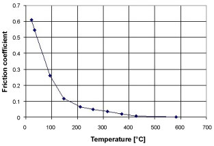
The main interaction in the model is the friction between the plate and the tool surfaces. The work pieces and the tool probe and shoulder are assumed to experience frictional contact described by Coulomb's frictional law with temperature dependent coefficient, μ. Coulomb's law is represented by the expression $F_f=\mu \cdot F_n$, where F_f is the local friction force and F_n is the normal force applied to the work piece [26]. The temperature dependence of the friction coefficient is shown in Figure 4 [27]. The friction sliding between the plate and the tool surfaces is a source of heat. The fraction of dissipated energy converted into heat, ${\eta }_f$, and the weighting factor, f_f, for distribution of the heat between the interacting surfaces can be specified in the interaction module of ABAQUS/CAE. In the beginning these parameters are set to 1 and 0.9 respectively, which indicates that all of the dissipated energy is converted into heat and 90% of this heat flows into the plate surface and 10% flows into the tool surface. It is worth mentioning that these parameters should be subsequently adjusted by comparing the results of the simulation with experimental data.

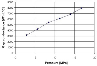
The conductive heat transfer between contact surfaces is assumed to be defined by $q_{ht}=k({\theta }_A-{\theta }_B)$, where $q_{ht}$ is the heat flux per unit area crossing the interface from point A on one surface to point B on the other surface, θ_A and θ_B are the temperatures of the points on the surfaces, and $k$ is the gap conductance. For the interaction of the tool surface with the plate surface gap conductance is defined as a function of contact pressure. Figure 5 shows this pressure dependence, the values of which are taken from [28].

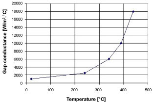
The anvil of the model dissipates heat without suffering deformations. Thus the gap conductance for the heat transfer between the plate and the anvil has only temperature dependence, which is represented in Figure 6. These thermal conductance values are taken from [23].

Finally the heat loss to the ambient air is modelled subjecting all the free surfaces of the model parts to surface convection interaction represented by the function $q_c=h\left(\theta -{\theta }^0\right)$, where $q_c$ is the heat flux per unit area in the direction of the outer normal unit vector, $\theta$ is the temperature of the part, ${\theta }^0$ is the room temperature (sink temperature) and h is the film (convection) coefficient, which are set to 25 ℃ and 15 W/(m2· ℃) respectively.

Boundary conditions

Several boundary conditions are applied to the different parts of the model in order to simulate the FSW with accuracy.

In the model of this study the anvil is only used to dissipate heat. Thus the displacement of the anvil is restricted in all directions to make it non-deformable and the bottom surface of the plate is also fixed in all directions. The clamps that prevent the plates from moving and separating during welding are taken into account by applying boundary conditions that restrict displacement of the longitudinal faces of the plates in all directions.

Regarding the initial temperatures of the parts, they are set to 25 ℃ representing that all the parts are at the room temperature at the beginning of the process.

Gravity load of 9.81 m/s² is applied to the whole model too.

Simplified models

Throughout the study the model described in previous sections was simplified in order to reduce the high computational cost of its simulations and the excessive element distortion problems. The present section explains the simplified models used during the study, which make it possible to know the effects of several parameters on the results of the simulations and at the same time, reduce computational cost. The first simplification lies in removing the anvil and replacing it with a boundary condition that simulates the contact conductance between the plate and the anvil itself. The number of elements of the model is also reduced by using a small plate of 40 × 40 × 5.85 mm instead of the real one. It permits to simulate the first three steps of the model described before, but not the second step of the weld period because the tool would come out of the plate.

The plunge period is hard to simulate because of the large deformations in the plate, which has not increased its temperature yet. Another simplified model is used to simulate the FSW process without simulating the first period. The plate of this model has a hole of the probe dimensions and the first step of the model is the dwell period of the FSW process. Thus the shoulder of the tool is in contact with the plate from the beginning of the simulation. Another option is used in order to reduce the computational time of the simulation of the first step (plunge period). This option lies in increasing the plunge feed rate. Thus the length of the plunge period is reduced.

Finally a last simplified model is built to make it possible to simulate the plunge period completely without excessive element distortion problems. In this model the plate thickness is reduced to 2 mm. The tool needed to weld 2 mm thickness plates is smaller than the tool described above. Thus the diameters of the probe and the shoulder are reduced to 3 mm and 10 mm respectively, and the probe length is reduced to 1.5 mm. This model also uses the "small plate" simplification detailed above and, even though the anvil is not replaced, its dimensions are reduced in keeping with the small plate dimensions. Plunge feed rate is also increased in this simulation, but not as it was explained above. In this model the plunge period lasts 1.9 seconds and the plunge feed rate has two values, 2.67 mm/s during the first 0.3 seconds of the period and 0.49 mm/s during the remaining 1.6 seconds.

Results and Discussion

Simulations from 2^nd step

As it was explained, the high computational costs of the analyses resulted in some simplifications of the FE-model. One of the options to reduce the computational time is to begin the simulation of the FSW process from the dwell period (2^nd step). This section presents all the results from the simulations with this option. Other simplifications explained in previous sections, such as working with a small plate or replacing the anvil, are also used in order to obtain the results.

Different tool shapes

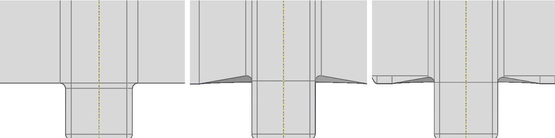
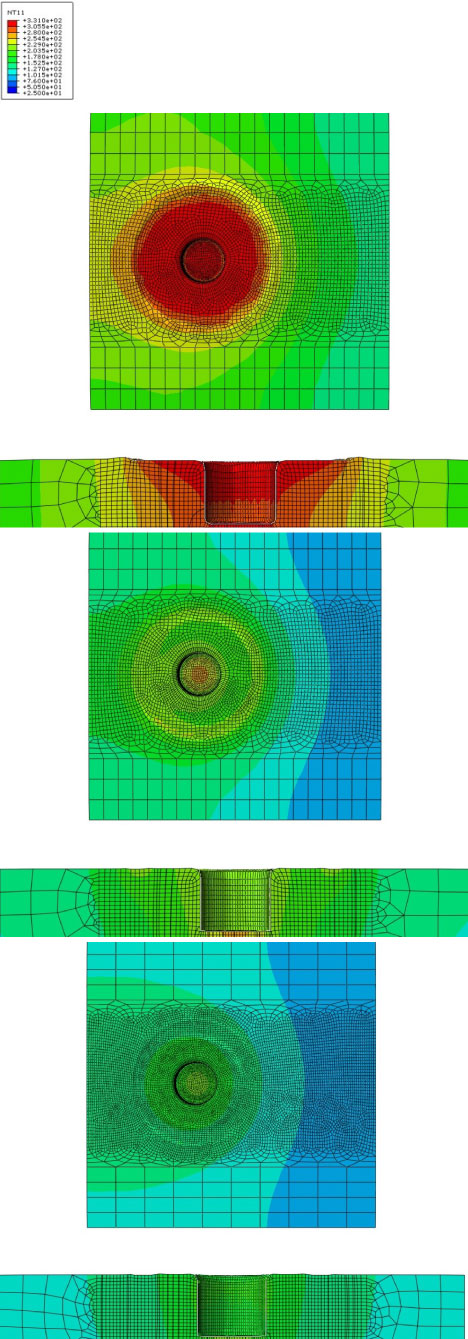
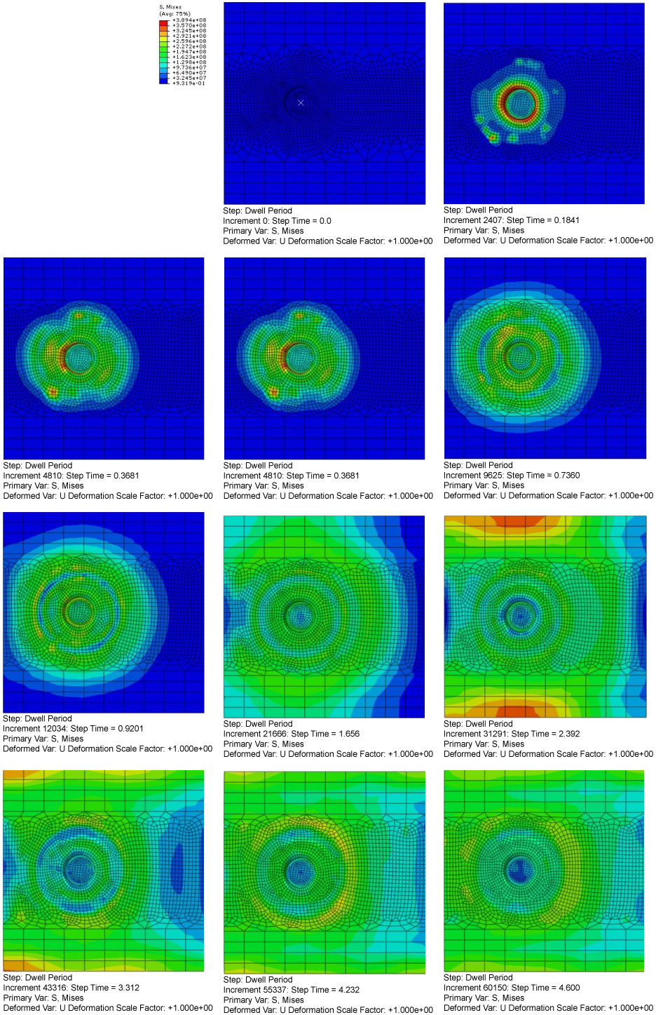
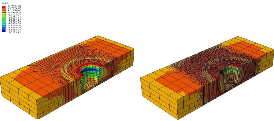
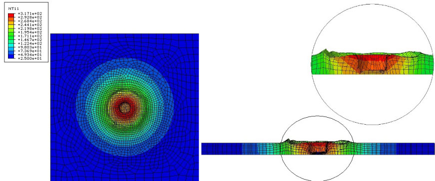
Tool technology is a factor of vital importance in FSW processes. Many aspects take part in the tool design, but tool geometry is one of the most important features. This section shows the results of three simulations which enable to compare three different tool geometries. The shape of the probe is the same in all the simulations, whereas the shoulder is changing from a flat surface to a concave surface with a chamfered perimeter. Figure 7 shows the different tool shapes used in the simulations.

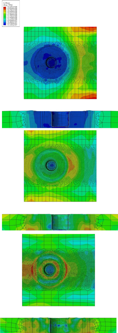
Figure 8 and Figure 9 illustrate contour plots of the equivalent von Mises stress and the nodal temperature at the end of the dwell period respectively. These figures show contour plots of the top surface and the lateral crosscut through the plate at the tool centre. The same order as Figure 7 is followed in Figure 8 and Figure 9, therefore, for example, illustrations designated with a) are results from simulations with the tool shape designated with a) in Figure 7.

The vertical displacements of plate nodes at the end of the second step are shown in Figure 10 in order to make it easier to compare the deformation of the plate with the different tools.

Comparing Figure 8, Figure 9 and Figure 10 it can be noticed that there is a great difference between the results obtained from the simulation which uses a tool with a flat shoulder and the results obtained by using the other tool shapes with a concave shoulder, which are quite similar. This difference results from the area of shoulder surface that makes contact with the plate, which is much larger with the first tool shape than with the other two tool shapes, since the simulations begin from dwell period and the plunge period is excluded. Thus, heat flux due to friction is higher in the first case, which increases the temperature of the plate. By using the tool with the flat shoulder the equivalent von Mises stresses under the tool shoulder are lower, as the material goes soft and the friction force decreases due to the temperature dependent friction coefficient, whereas, for the same reasons, deformation is higher.

Instantaneous or ramped up rotational velocity

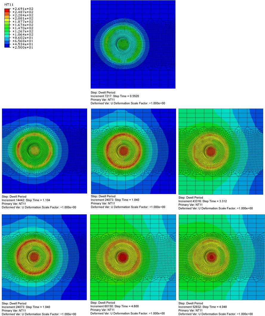
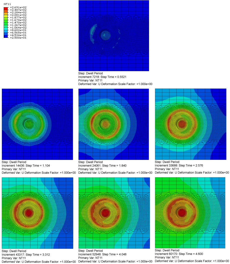
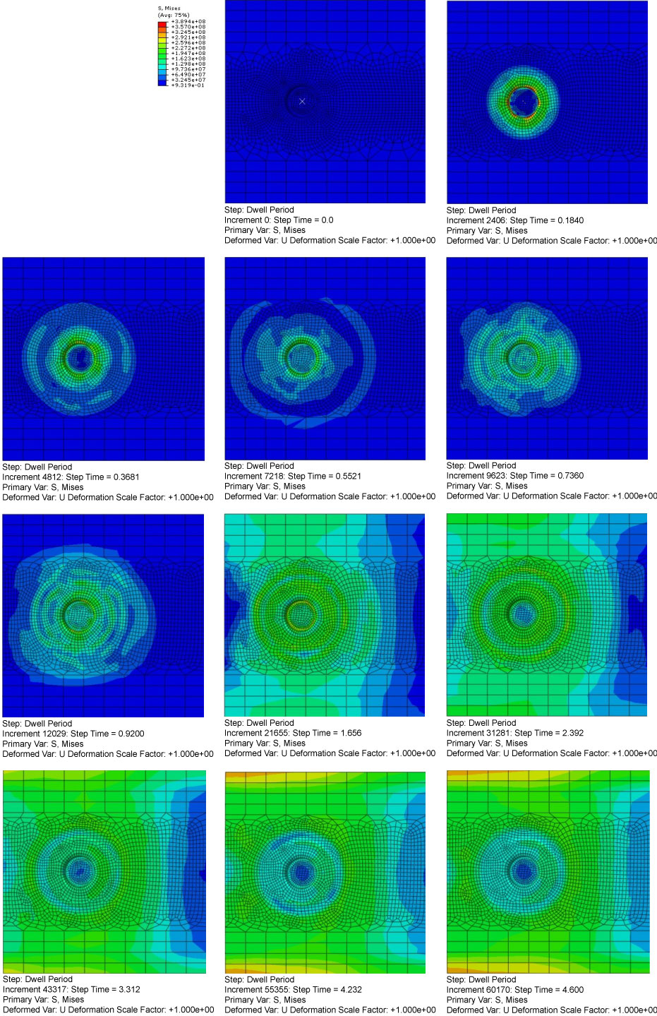
The rotational velocity of the welding tool can be applied in two different ways. On the one hand, it can be applied as an instantaneous velocity. On the other hand, the velocity can be ramped up smoothly from zero to the set rate. The following section shows the differences that appear in the simulation results by using these two options. Figure 11 and Figure 12 are two sequences of contour plots of the nodal temperature throughout the dwell period that illustrate the evolution of the temperature of the plate by using instantaneous and ramped velocity respectively.

Comparing Figure 11 and Figure 12 it is seen that temperature rises faster with instantaneous rotational velocity and it causes a strange phenomenon, since temperature of the contact zone decreases from the 2^nd second, whereas using a ramped rotational velocity it increases regularly all the time.

The differences in the equivalent von Mises stress evolution can be appreciated in the sequences of Figure 13 and Figure 14.

In Figure 13 it also can be seen that instantaneous velocity causes an impact phenomenon, which leads to strange results.

The results shown in the sequences on Figure 11, Figure 12, Figure 13 and Figure 14 make it possible to realize that, when the simulations begin from the dwell period, it is necessary to use ramped rotational velocity in order to obtain accurate results.

Mesh effects

Another important factor to obtain reliable results is the quality of the mesh. The results may vary quite a lot depending on the accuracy of the mesh, which should be considerably high, above all in the welding zone. The aim of the present section is to compare two different meshes. The element type and mesh controls are the same for both meshes, the only difference is that the first mesh is coarser than the second one in the welding zone. The used meshes have 21,881 and 160,928 elements respectively.

The distribution of the nodal temperature at the plate at the end of the dwell period can be compared in Figure 15.

Contour plots of the equivalent von Mises stress of both meshes are presented in Figure 16. These illustrations are also taken at the end of the dwell period.

The vertical displacements of plate nodes at the end of the second step are shown in Figure 17 in order to make it easier to compare the deformation of the plate.

Figure 15, Figure 16 and Figure 17 show the great differences between the results obtained from the simulations with different meshes. Thus, it would be very important to verify the results with experimental data and find a suitable mesh to obtain accurate results with the minimum computational cost.

Simulations from 1^st step

When the plunge period is included in the FE-model the simulations become very complicated and fail due to excessive element distortion. However some interesting results are presented in this section beginning the analyses from the first step.

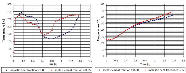
Inelastic heat fraction effects

The inelastic heat fraction, η, is an interesting parameter of the model. Two models are simulated in order to analyse the effects of varying the value of this parameter. In the first model inelastic heat fraction is set to 0.8, whereas in the second model is increased to 0.95. In both models the plunge feed rate is increased in order to reduce the plunge period length to 2 s. This simplification makes it possible to reduce the computational time and know the effects of the change of this parameter. Despite the simplification, the evolution of the temperature values can be studied, although the magnitudes may differ from the results from a simulation with the real plunge feed rate. The evolutions of the temperature at two points of the top surface of the plate are presented in two graphs (see Figure 18). One graph shows the evolution of the temperature at the point of the plate which is situated at the centre of the probe, whereas the other one is a graph of the evolution of the temperature at a point of the joint line situated outside the projection of the tool shoulder.

Figure 18 shows how temperature rises when inelastic heat fraction increases, since the greater inelastic heat fraction is, the more heat flux due to plastic deformation appears. It is worth mentioning that in Figure 18a it should be neglected the first 0.75 seconds, as they are from a transient state, which is caused by the use of instantaneous rotational and vertical velocities instead of ramped velocities. It can be concluded that inelastic heat fraction is an important parameter for the simulations of FSW processes and, however it is set between the recommended limits (0.8-1) in the present study; it should be further adjusted by verifying the obtained results of the complete simulation with experimental data.

Plunge period

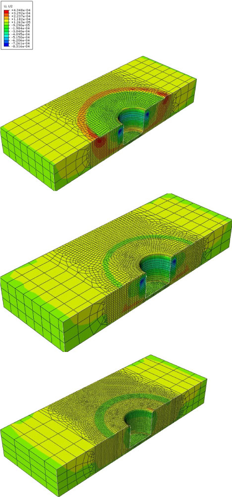
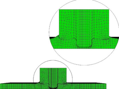
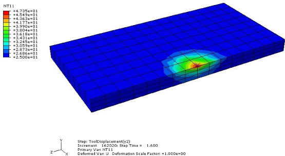
The simulation of the last simplified model presented in section 3.6 makes it possible to have results of the entire plunge period, although the features of the model are different from the experimental data followed to build the main model of the study. The following figures illustrate the results obtained from the analysis of the model with, among others, the 2 mm plate simplification. First of all, a lateral crosscut through the plate at the tool centre is presented in Figure 19 in order to show the deformed shape of the model at the end of the plunge period. The figure enables to see how the material of the plate is displaced from its initial position and fills the space under the concave shoulder. It is important in order to keep the pressure under the tool shoulder.

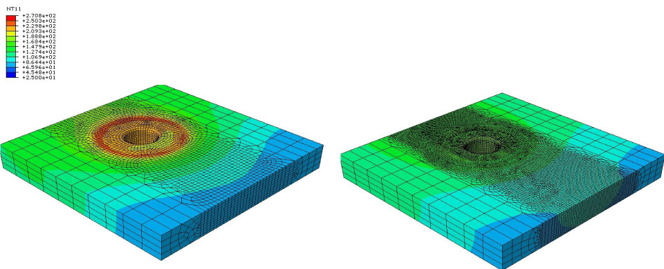
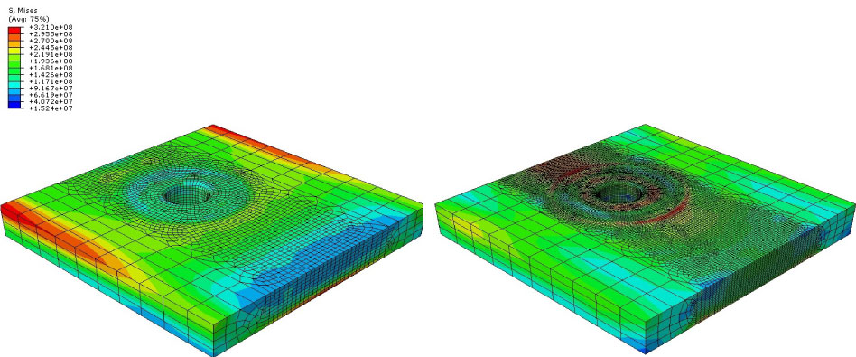
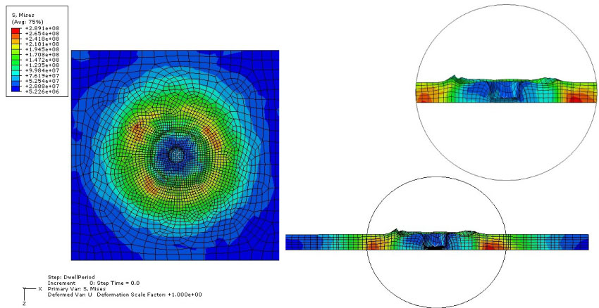
The magnitude of the equivalent von Mises stress at the end of the plunge period is shown in Figure 20. In this figure the anvil is removed because it does not suffer any stress due to the boundary conditions applied to the model (see section 3.5). Figure 21 and Figure 22 show the temperature distribution in the model at the end of the plunge period.

The anvil is removed in the Figure 1; however, its temperature distribution is illustrated in Figure 22 using different scale limits. Those figures make it possible to see that the zone under the tool shoulder reaches the highest temperatures, which makes the material of this zone to go soft and reduces the equivalent von Mises stress due to the temperature dependent material properties.

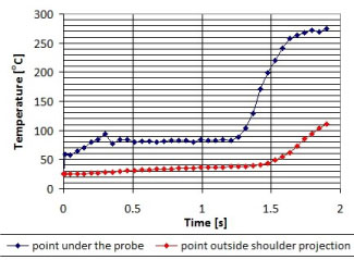
Finally, Figure 23 shows the evolution of the temperature at two points of the top surface of the plate. One of the points is situated under the probe and the other one is situated outside the zone of the shoulder projection. It is important to notice that temperature of the plate begins to rise considerably at the 1.3 seconds, when the material of the plate has come up enough to establish contact with the tool shoulder. It could be considered as the beginning of the dwell period.

Conclusions and Future Work

The complete simulation of the Friction Stir Welding process by using the finite element software ABAQUS 6.9-EF1 turned out to be unachievable in the present study. However, the previous model [10] was improved by adding the welding tool as a physical rigid body. Besides, a fully coupled thermo-mechanical analysis was used instead of a sequentially coupled thermo-mechanical analysis. The simulations were not completed due to excessive element distortion and high computational cost, even though several techniques, such as ALE meshing technique and mass scaling, were included to the model in order to solve these problems. Despite any simulation of the entire FSW process was achieved, this study made it possible to analyse and check several aspects. It was proved that tool geometry has a vital importance in the FSW process. The influence of using instantaneous or ramped velocity at the beginning of the simulations was studied too. Moreover, it was also seen that the mesh used in the finite element analysis and the adjustment of the inelastic heat fraction have a great influence on the obtained results.

The first goal that this study leaves for a future work is to complete the fully coupled simulation of the FSW process. In order to achieve this goal, new aspects introduced in this study, such as ALE meshing and mass scaling techniques, should be further investigated and developed. If a completed simulation of the FSW process was achieved, it would be possible to analyse other parameters and features in order to develop this welding technique. It would be interesting to compare the three tool shapes studied in section 4.1.1 again, but in the plunge period instead of the dwell period. In this way, the function of the concave shoulder could be seen much better. There should be also more attention to the interaction properties between the tool, the plate and the backing plate, which play a significant role in the welding process. Thus, these properties should be adjusted by verifying the results of a completed simulation with experimental data. Once the interaction properties adjusted, the results obtained from the simulation of the model would be reliable and several welding parameters, such as different traverse and rotational velocities and different plunge feed rates, could be tried to see the changes of the stresses and temperature distributions and improve the welding process. Tool tilt angle is an important feature of the FSW process which was neglected in the present study. Thus, it would be interesting to further include it in the model. Then, the process could be simulated with different values of this parameter in order to see its effects on the weld. Finally the extraction of the tool and the cooling phase of the FSW process could also be included to the model to calculate the residual stress distribution.

References

1. TWI (2010) Friction Stir Welding-Intellectual Property Rights.
2. Mishra RS, Ma ZY (2005) Friction stir welding and processing. Materials Science and Engineering R: Reports 50: 1-78.
3. Zhang YN, Cao X, Larose S, et al. (2012) Review of tools for friction stir welding and processing. Can Metall Q 51: 250-261.
4. Galvão I, Leal RM, Rodrigues DM, et al. (2013) Influence of tool shoulder geometry on properties of friction stir welds in thin copper sheets. J Mater Process Technol 213: 129-135.
5. Biswas P, A Kumar D, Mandal NR (2012) Friction stir welding of aluminum alloy with varying tool geometry and process parameters. Proc Inst Mech Eng Part B J Eng Manuf 226: 641-648.
6. Khodaverdizadeh H, Heidarzadeh A, Saeid T (2013) Effect of tool pin profile on microstructure and mechanical properties of friction stir welded pure copper joints. Mater Des 45: 265-270.
7. Imam M, Biswas K, Racherla V (2013) Effect of weld morphology on mechanical response and failure of friction stir welds in a naturally aged aluminium alloy. Mater Des 44: 23-34.
8. Mehta M, De A, DebRoy T (2014) Material adhesion and stresses on friction stir welding tool pins. Sci Technol Weld Join 19: 534-540.
9. Mehta M, Reddy GM, Rao AV, et al. (2015) Numerical modeling of friction stir welding using the tools with polygonal pins. Def Technol 11: 229-236.
10. Gagner J, Ahadi A (2009) Finite element simulation of an AA2024-T3 friction stir weld. Int Rev Mech Eng 3: 427-435.
11. G Buffa, J Hua, R Shivpuri, et al. (2006) Continuum based fem model for friction stir welding-model development. Mater Sci Eng 419: 389-396.
12. HW Zhang, Z Zhang, JT Chen (2007) 3D modeling of material flow in friction stir welding under different process parameters. J Mater Proc Tech 183: 62-70.
13. Z Zhang, JT Chen (2008) The simulation of material behaviours in friction stir welding process by using rate-dependent constitutive model. J Mater Sci 43: 222-232.
14. Buffa G, Hua J, Shivpuri R, et al. (2006) Design of the friction stir welding tool using the continuum based FEM model. Mater Sci Eng A 419: 381-388.
15. YH Xiao, Zhan HF, Gu YT, et al. (2016) Modeling heat transfer during friction stir welding using a meshless particle method. Int J Heat Mass Transfer 104: 288-300.
16. Jain P, Pal SK, Singh SB (2016) A study on the variation of forces and temperature in a friction stir welding process: A finite element approach. J Manuf Proc 23: 278-286.
17. M Lepore, P Carlone, F Berto, et al. (2017) A FEM based methodology to simulate multiple crack propagation in friction stir welds. Eng Fract Mech 184: 154-167.
18. Aziz SB, Dewan MW, Hugget DJ, et al. (2018) A fully coupled thermo mechanical model of friction stir welding (FSW) and numerical studies on process parameters of lightweight aluminum alloy joints. Acta Metallurgica Sinica 31: 1-18.
19. Cambridge University (2002) FSW Benchmark.
20. ABAQUS version 6.9-EF1 documentation.
21. Ellad B Tadmor, Ronald E Miller, Ryan S Elliott (2012) Continuum mechanics and thermodynamics- from fundamental concepts to governing equations. Cambridge University press.
22. (1990) Properties and Selection: Nonferrous Alloys and Special-Purpose Materials, USA.
23. Q Shi, T Dickerson, HR Shercliff (2003) Thermo-mechanical FE modelling of friction stir welding of Al-2024 Including Tool Load. Proceedings of the 4^th Symposium on Friction Stir Welding, Park City, Utah, ISA, 14-16.
24. H Schmidt, J Hattel, J Wert (2004) An analytical model for the heat generation in friction stir welding. Modelling Simulation Mater Sci Eng 12: 143-157.
25. Gregory Kay (2003) Failure modeling of titanium 6Al-4V and aluminum 2024-T3 with the Johnson-Cook Material Model. Federal Aviation Administration Report.
26. Hot Work Steels, AISI H13 (DIN 1.2344) EFS, Fletcher Easysteel, 51-53.
27. M Awang, VH Mucino, Z Feng, et al. (2005) Thermo-mechanical modeling of friction stir spot welding (FSSW) process: Use of an explicit adaptive meshing scheme. SAE International 01-1251.
28. H Yuncu (2006) Thermal contact conductance of nominaly flat surfaces. Heat Mass Transfer 43: 1-5.