Journal of Fluid Dynamics

Influence of the Downstream Vehicle Length on Train Aerodynamics Subjected to Crosswind

Abstract

Limited by the wind tunnel size, a short-length train model is generally adopted during the test to represent the realistic long tandem. Thus, the reasonable arrangement of the trailing vehicle is of significance for experimental accuracy. In this work, the aerodynamic performance of the trains with different downstream vehicle lengths subjected to crosswind is studied using the improved detached eddy simulation (IDDES) method combined with the Shear-Stress-Transport k-ω turbulence model. Wind tunnel models of high-speed train with five different downstream trailing lengths are proposed to represent typical cases in the wind tunnel at the yaw angle ranging from β = 0° to 60°. Results show that the aerodynamics and flow patterns of the L^a = 0.50 and 3-unit car cases are highly relevant. The downstream dummy body length has the greatest effects on aerodynamic coefficients at higher yaw angle (β > 30°), especially at β = 60°, whereas the effects become insignificant at lower yaw angle (β < 30°). For various L^a lengths, the notable discrepancies appear at leeward and top sides where large vortexes shed off from the roof. The larger contributions to the lateral force and lift force coefficients are mainly due to these areas. A suitable length of L^a = 0.50 is therefore recommended to obtain more accurate aerodynamics of the long train set.

Keywords

High-speed train, Crosswind, Downstream dummy vehicle

 Introduction

Currently, methods for studying train aerodynamic characteristics include physical model tests (e.g., full-scale test, wind tunnel test, moving model test) and numerical simulation [1]. With the rapid development of computer resources, computational fluid dynamics (CFD) has developed rapidly recently and more intensive methodologies are increasingly used such as RANS, PANS, LES, and DES [2,3]. The turbulence models of numerical simulation, however, are based on fundamental assumptions and the results are essentially approximate solutions. Thus, the numerical simulation is extremely dependent on test verification and calibration.

The three methods mentioned above can complement and reinforce each other and jointly develop. However, for the wind tunnel test, due to its irreplaceable advantages, has been in the leading position for studying and predicting the flow distribution and mechanism around the train, in the past and now. Although there are some limitations of wind tunnel tests, such as the support and wall interference and the inability to simulate relative motion, it has its own superiority that other methods cannot be compared with. It can not only provide a verification basis for numerical simulation but also the flow parameters, such as the temperature, humidity, and velocity can be easily controlled because of the indoor test conditions [4-6]. It can perform the accurate and repeatable measurements and is more convenient than full-scale test. Therefore, the wind tunnel test has become one of the most important and extensively used methods for studying train aerodynamic performance at present.

The train has the shape features of slim & slender body with long length, which is quite different from those objects like automobiles and buildings. The general blockage ratio of the wind tunnel for train model is far less than 0.5% under crosswind. The key factor restricting the train wind tunnel tests for various yaw angles, however, is deemed to be the length of the train. The wind tunnel tests of trains are usually conducted at high Reynolds number conditions, which demand a higher test speed. However, the high-speed test section of the wind tunnel usually has a narrower test section due to the limited driving power and total energy. At larger yaw angles, however, train models with large scale (e.g., 1:8) demand much longer and wider test sections. Due to the limited dimensions of the wind tunnel test section, especially the width direction, researchers would have to use a short-unit train (3-cars) instead of a real train (8-cars, 16-cars) to conduct wind tunnel tests subjected to crosswind. Even for a 3-unit train with a 1:8 scale, it would be impossible to conduct wind tunnel tests at a yaw angle larger than 30° in some circumstances [7]. Therefore, it is of great significance to study the selection of a shorter train model in the wind tunnel test.

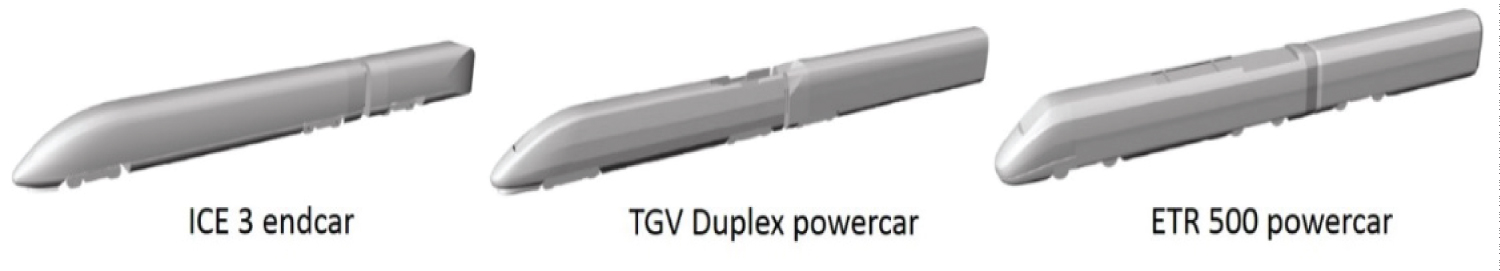
The aerodynamic performance of the leading vehicle is generally considered the worst among the 3-unit train under crosswind, therefore, the model with a full-length of the lead car and an additional half-car is usually recommended. The aerodynamic characteristics of the lead car are focused to represent the 3-unit train. It is specified in EN14067-6 that for all passenger vehicles and locomotives under investigation at least half a downstream vehicle shall be placed next to the tested model to ensure realistic flow around the rear of the leading vehicle [8]. Three wind tunnel benchmark vehicle models are given in Figure 1, they are ICE 3 endcar, TGV Duplex powercar and ETR 500 powercar. All vehicle models adopted a full length of the lead car and an additional downstream dummy body. However, the downstream dummy body are not unified, both in shape and length.

Researchers have conducted extensive wind tunnel campaigns using different lengths of the downstream vehicle. A 1/10^th-scale and a 1/25^th-scale model of Inter-City Express 3 (ICE3) were applied for assessing the slipstream of high-speed trains by wind-tunnel methodology, and the 1/10th-scale ICE3 train model contained just a lead car and a rear car [9]. A 1:10 scale ETR500 train model was measured through wind tunnel tests for different infrastructure scenarios, including flat ground with and without ballast and rail, and a 6m embankment, and for a typical Italian viaduct, the test model consisted of a lead car and a middle car [5]. An ICE3 model which consists of a lead car and half a streamlined body has been investigated in an automotive wind tunnel on three different ground configurations utilizing force measurements and flow visualization [10]. Experimental tests of a 1:10 scale model of the EMUV₂50, which was made up of a locomotive and 1/3 of the first trailer coach, have been carried out in [5]. An extensive experimental campaign has been carried out by [4] to measure the aerodynamic forces acting on rail vehicles subjected to crosswind, including ETR480, ETR500, and IC train with three car unit. The differences of wind-induced forces and pressures between moving model experiments and static experiments have been explored using a 1:25 scale model of a Class 390 Pendolino at a 30° yaw angle [11]. The train model comprised full reproduction of the leading car followed by a partial trailing car. Wind tunnel tests were carried out by [1] to investigate the pressure on the train and the overall side force per unit length over the yaw angle range from 15 to 30°. The train model consists of a 1/25^th scale model of the Class 43 power car and one trailing Mark 3 coach mounted on the ground board. Train models of CRH380A scaled at 1:8 and 1:20, both comprised of a streamlined lead car and a streamlined rear car, were employed by [6] in a wind tunnel to test the influence of the Reynolds number on the aerodynamic force and pressure of a train at yaw angles of 0° and 15°. The influences of wind angle on the train aerodynamics were investigated using a 1/8^th scale train model within 20 degrees of the wind angles [7]. The experimental model is a 3-unit CRH2 train (two streamlined cars and a middle car) with dismountable bogies and windshields. It can be seen from above that the train models employed in wind tunnel tests have all kinds of downstream body lengths, and the aerodynamic influence of the downstream vehicle on the lead car was not clarified yet.

The previous investigations about the train wind tunnel tests are mainly focused on the discussions and analysis of the data and results, whereas little attention is paid to the train model itself. Thus, the objective of the current work is to explore the influence of the downstream vehicle lengths on train aerodynamic characteristics. The simulations are performed using the IDDES method combined with the Shear-Stress-Transport (SST) k-ω turbulence model. The method employed in this study is firstly validated by previous research by comparing the aerodynamic coefficients of the head car. Then, train models with five different downstream body lengths are proposed to represent typical cases in the wind tunnel at the yaw angle ranging from 0° to 60°. The aerodynamic coefficients and the flow field around the lead car at a yaw angle of 60° where the largest discrepancy takes place are fully analyzed at last.

Numerical Simulation

Model description

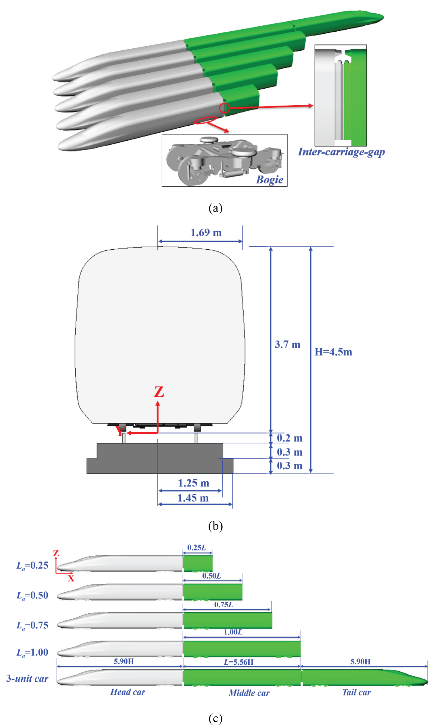
A 1/8^th scaled CRH380A high-speed train model was used in the simulation. The model scale is selected by referring to the model used in the previous wind tunnel tests [12]. For all geometry models, downstream dummy vehicles with different lengths are placed next to the head car, whose lengths are L^a = 0.25L, 0.50L, 0.75L, and 1.00L, respectively. Here L is the length of the full middle car. In addition, a 3-unit car which consists of a lead car, a middle car, and a tail car is also simulated as the benchmark for other cases. As is shown in Figure 2, the train model is 3.38 m in width and 3.7 m in height in full scale, with a cross-sectional area of 11.22 m2. Figure 2 also shows the definition of the coordinate system (x, y, z), with the origin point mounted at the train nose on the rail level and the center of the tracks.

The distance between the roof of the train and the rail level is 3.7m. Since the ballastless rail is universally adopted in high-speed railways in China, in consideration of typical representative, a single-track ballastless rail was employed in this study, which differs from that specification of EN 14067-6 [8]. The distance between the roof of the train and the ground is H = 4.5 m, which is adopted as the characteristic dimension. Based on the wind tunnel tests, some details were considered including the bogies and inter-carriage gaps. Note that the wheel of the bogie was flattened to avoid contact with the rail, and a 5 mm separated gap of the windshield was adopted to avoid contact and vibration with the adjacent vehicles, which are common practices in wind tunnel tests.

Numerical method

Aerodynamic loads experienced on the train in the wind tunnel test are essentially unsteady phenomenon due to the intrinsic unsteadiness of turbulent flow. However, the mean aerodynamic loads acting on the train are usually more concerned. It is therefore possible to use the IDDES method based on the shear stress transport (SST) k-ω turbulence model embedded within its RANS part was applied [13]. The shear-stress transport (SST) k-ω model is chosen as the turbulence closure model for its ability to solve a complex flow with large separations and adverse pressure gradients [14]. The SST model incorporates a damped cross-diffusion derivative term in the ω equation. The definition of turbulent viscosity is modified to account for the transport of the turbulent shear stress [15]. These features make the SST k-ω model more accurate and reliable for a wider class of flows (for example, adverse pressure gradient flows, and airfoils) than the standard k-ω model. Perhaps the most significant advantage, however, is that the model can be applied throughout the boundary layer, including the viscous-dominated region, without further modification [16]. In the spatial discretization methods, a second-order upwind scheme was used for the convective term, turbulent kinetic energy term, and specific dissipation rate term. The SIMPLE method was adopted for coupling the pressure-velocity field, and an iterative method was used to correct the pressure. The physical time-step of the unsteady calculation was set as ∆t = 5 × 10^-5s, within 30 inner iterations to ensure all residuals drop by at least one order of the magnitude in each physical time step. The commercial CFD code of Fluent 18.2 was employed to solve the whole issue.

Computational domain and boundary conditions

The computational domain of 3-unit car case is shown in Figure 3 below. According to EN-14067-6, the computational domain boundaries shall not interfere with the flow around the vehicle in a physically incorrect way. The computational domain in this work is 54H (length) × 27H (width) × 11H (height), where H is the characteristic height described in section 2.1. The width of the domain is divided as 9H on the windward side and 18H on the leeward side. The domain extends in the streamwise direction, for 12H upstream and 24H downstream relative to the train, which is sufficient to meet the requirements of the norm [11].

Based on the wind tunnel tests that the relative motion is unable to simulate, the boundary conditions are specified as follows: the velocity inlet boundaries are applied both for the front side and the windward side of the domain, and the pressure outlets boundaries are added for leeward side and back side of the domain. All the boundaries of the train model are treated as no-slip walls, so as the stationary ground, the rail, and the subgrade. The top of the domain is set as a symmetry condition.

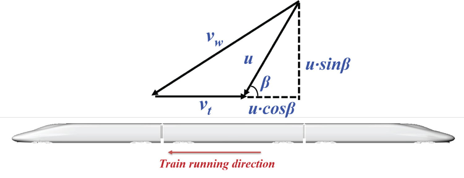
The crosswind is simulated by the resultant method. Figure 4 shows a schematic of the train running under crosswind, where v_w is the wind speed, v_t is the train speed, and u is the resultant wind speed relative to the train. The β marked in the figure is the yaw angle, which reflects the coupling relationship between the ambient wind speed and train speed [17]. In this work, the resultant wind speed u is kept constant at 60 m/s with a uniform profile whilst the inlet speed normal to the windward side (i.e. usinβ) and front side (i.e. ucosβ) are varied to simulate different yaw angles. Based on the resultant wind speed u and characteristic height H and kinematic viscosity ν (Re = uH/v), the corresponding Reynolds number (Re) is 1.9 × 10⁶, which is far higher than the minimum Re (2.5 × 10⁵) recommended by [8]. The blockage ratio in this paper is 0.2%, which is below 5% specified by [8], thus the results need no further correction.

Mesh setup and data processing

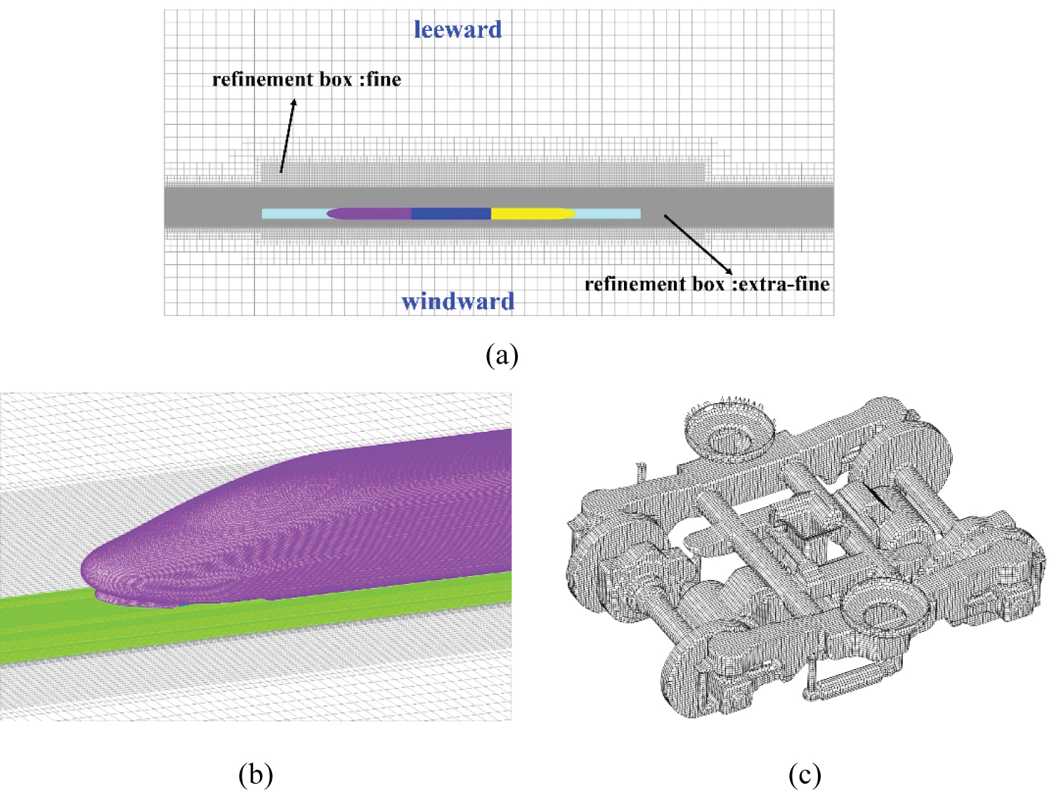
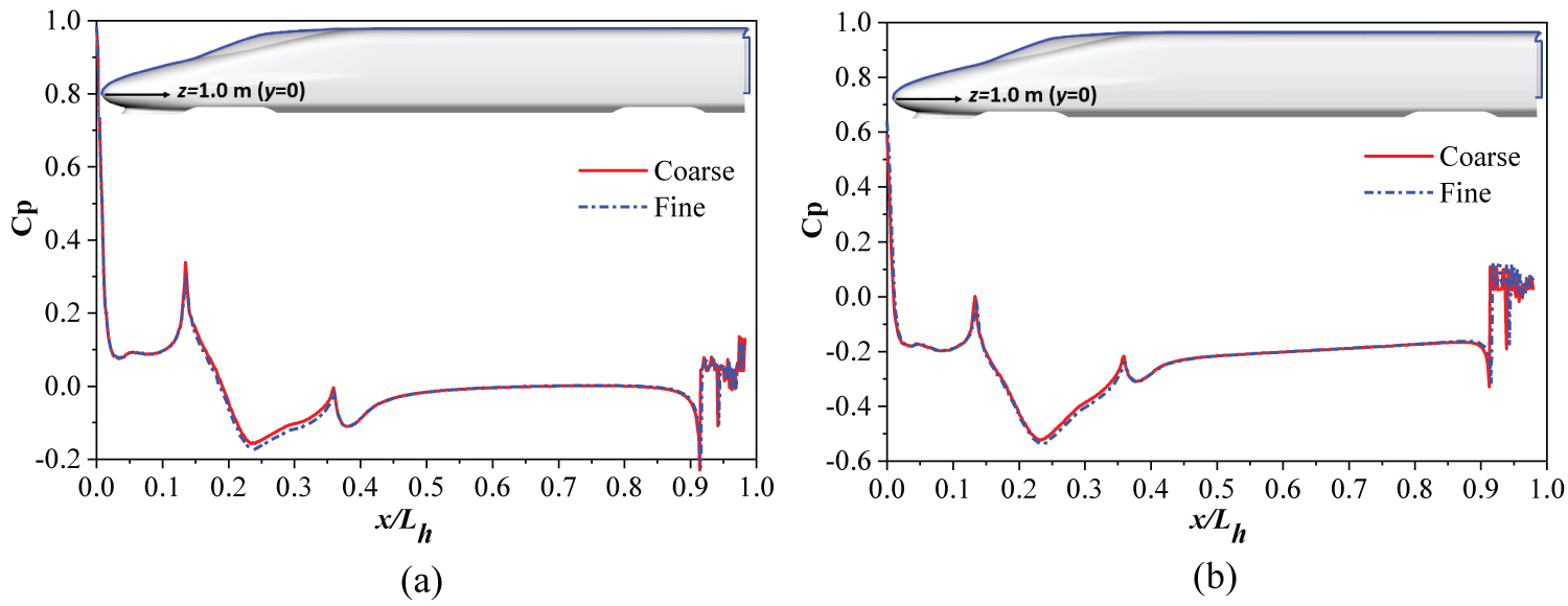
The gird was generated by the toolbox of Snappy HexMesh in Open FOAM 3.0. Two sets of grids are conducted to test the grid sensitivity, namely, coarse and fine mesh, which are 20 million and 36 million, respectively. Figure 5 shows details of the coarse mesh, two refinement boxes regions are added around the train to capture the turbulent flow details near the train. The extra-fine refinement box extended throughout the streamwise direction, 3.0H from the top of rail in the vertical direction, 1.5H from the center of the track on the windward side and 3.0H from the center of the track on the leeward side. The fine refinement box extended 4.0H ahead of the head car, 10H behind the tail car, 6.0H above the rail level, and 3.0H from the center of the track on the windward side and 6.0H from the center of the track on the leeward side. The computational domain is treated with mixed grids, with prism layers at the wall boundaries and hexahedral grids in the rest of the domain, as is shown in Figure 5. To guarantee the correct velocity gradient along the normal direction of the wall surface, 10 prism layers are performed to the train surface, with the first layer thickness of 0.20 mm. Thus, the y plus is within 30-50, which can meet the method requirements. Grid sensitivity tests are carried out at yaw angles 0° and 15°, the lateral force and lift force of these two meshes are shown in Table 1. The static pressure coefficients at position y = 0 on the top of the 3-unit train surface are shown in Figure 6. It can be seen that the static pressure coefficients of the two meshes differ little except in the region of the cab window area, and the error of the aerodynamic coefficients of the head car are all below 5%, indicating that the coarse mesh adopted in this work afterward is adequate to produce the results presented below.

The non-dimensional aerodynamic forces, including side force coefficient C_Fy, lift force coefficient C_Fz, rolling moment coefficient C_Mx, together with the static pressure coefficient C_p are defined as follows:

C_Fy= F_y/(0.5ρU_m²S) (1)

C_Fz= F_z/(0.5ρU_m²S) (2)

C_Mx= M_x/(0.5ρU_m²Sl) (3)

C_p= (P-P₀)/(0.5ρU_m²) (4)

where F_y, F_z, and M_x are the side force, lift force and rolling moment, respectively. The air density ρ is equal to 1.225 kg/m³. In addition, U_m is the composed wind speed, which is 60 m/s here and the reference area S is considered to be 11.22 m². The reference pressure P₀ is considered as 0 Pa. Further, l is the reference height of the rolling moment, which is 1.8 here based on the half train height.

Model Verification

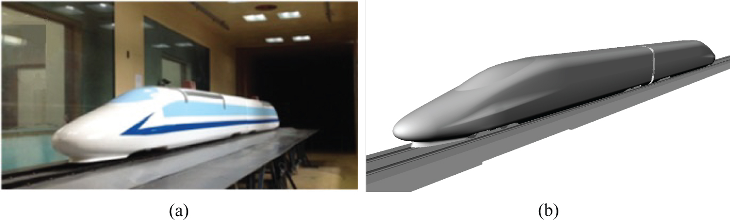
To verify the validity of the numerical algorithm adopted in this study, the present method was applied to compute the aerodynamic loads of the wind tunnel tests performed by [6]. A 1/8^th scale CRH 380A train model consisting of two cars was placed on an STBR scenario, with the incoming wind speed set at 60 m/s. The train models of the wind tunnel and numerical simulation are shown in Figure 7. The Reynolds numbers of the wind tunnel test and the numerical calculation are both equal to 1.9 × 10⁶ based on the wind speed and the characteristic height H of the train model. More detailed information about the wind tunnel setups can be found in [6]. The comparisons of the computational results and the wind tunnel data are listed in Table 1. The typical case of yaw angle 15° is selected, and the aerodynamic side and lift force coefficients of the head car are concentrated.

It was shown that the numerical results have a reasonable agreement with those of wind tunnel tests. The error of C_Fy between the numerical simulation and the wind tunnel test was 7.83%, while the error of C_Fz between the numerical simulation and the wind tunnel test was less than 5%. The main differences were probably due to the support interferences at the train bottom in the wind tunnel tests which the CFD was not considered (Table 2).

Results and Discussion

Aerodynamic force coefficients

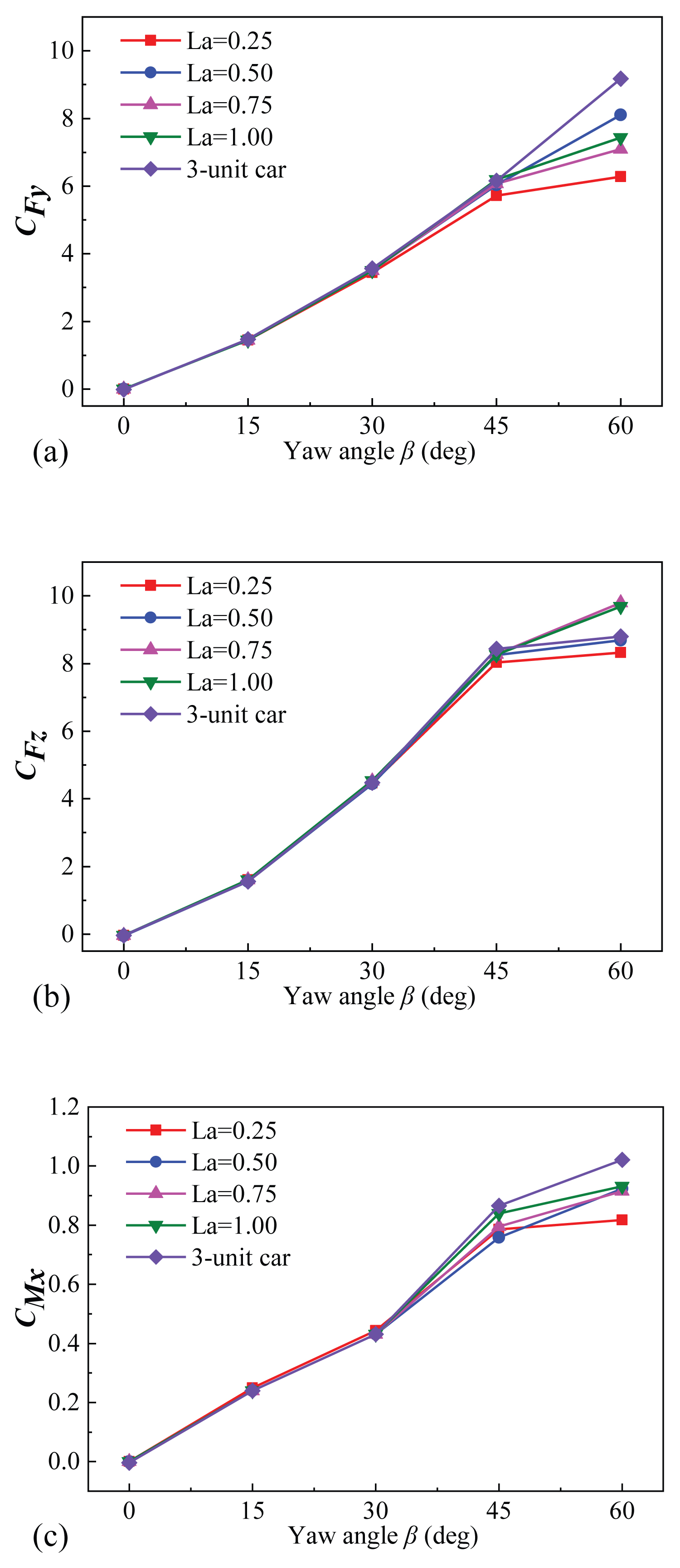
The side force (C_Fy) and the lift force (C_Fz) are the main causes of train derailment under crosswind [18]. Figure 8 presents the side force, lift force and rolling moment coefficients of the head cars with respect to various yaw angles up to 60 degrees. When the yaw angle β = 0°, the rolling moment and side force coefficients are nearly zero. This indicates that the incoming airflow is symmetric to the train body, thus no lateral load has occurred. When the yaw angle increases, the side force coefficients almost changed linearly with the yaw angle [19]. The lift force and rolling moment coefficients are positively increased significantly, indicating that growing uplift and moment are imposed on the train body, which exerts adverse impacts to train running safety [20].

In addition, two distinguished ranges are observed involving the yaw effects. When at lower yaw angles (β < 30°), the aerodynamic coefficients almost remain unchanged concerning the different downstream body lengths. The largest difference of C_Fy among different downstream body lengths is only 0.8% at β = 15°. At higher yaw angles (β > 30°), the aerodynamic coefficients under various downstream body lengths are more significantly sensitive to the yaw effects. The difference of these two regions on the aerodynamic coefficients represents two different flow behaviors, which may be called streamwise-dominant flow regime and detached-dominant flow pattern, respectively. At higher yaw angles, especially at β = 60°, when the downstream body lengths L^a increase, the overall change of C_Fy rises. However, no orderly rules of C_Fy are obtained, but with 3-unit car highest and L^a = 0.25 lowest, with a difference of 45%. The change of lift force C_Fz is more complicated at β = 60° involving different L^a. The most notable thing is that the C_Fz for L^a = 0.75 and L^a= 1.00 are close to each other and relatively greater, while the 3-unit car and L^a= 0.50 are approximately the same and showed a relatively lower value. In summary, the downstream dummy body length has the greatest effects on aerodynamic coefficients at higher yaw angle (β > 30°), especially at β = 60°, where the flow pattern is detached-dominant, whereas the effects become insignificant at lower yaw angle (β < 30°). Therefore, in the following passages below, the large yaw angle of 60° is chosen to analyze the aerodynamic performance with respect to the influence of downstream dummy body length.

Pressure distribution of the head vehicle (β = 60°)

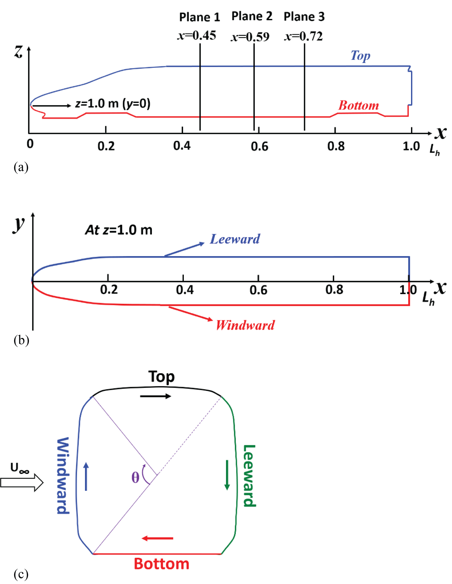
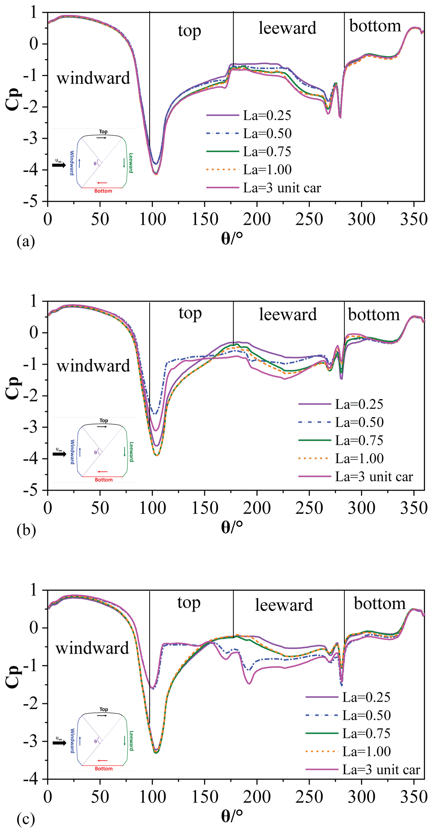
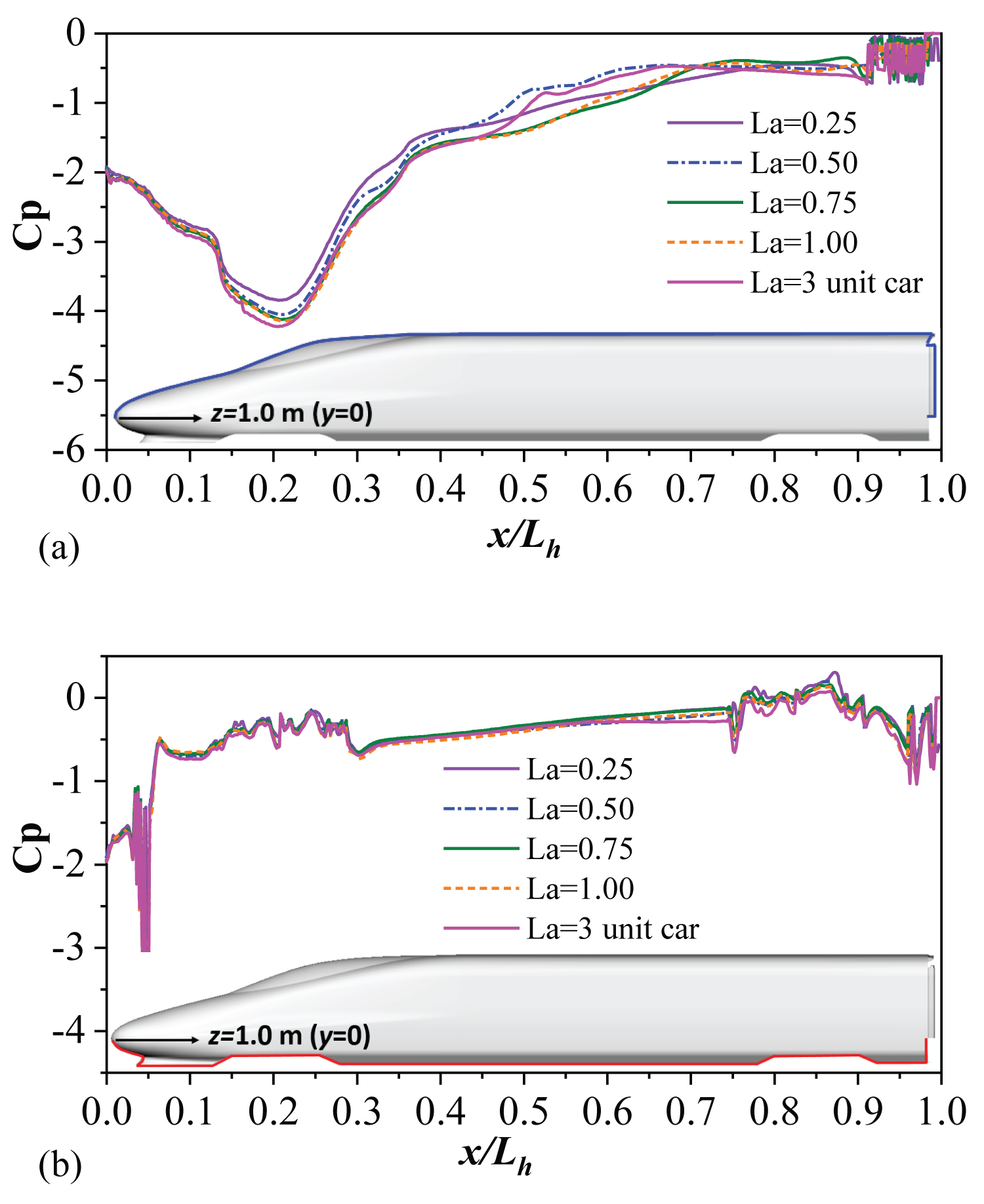
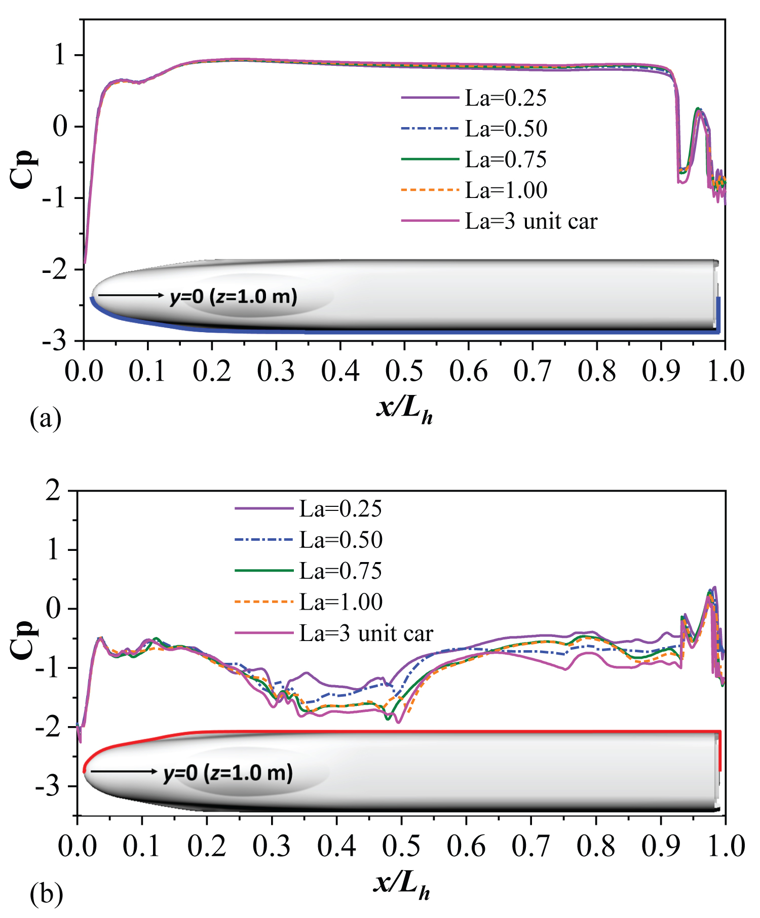
Since the train aerodynamic forces are obtained by integration of the surface pressure, it is necessary to explore the pressure distribution on the train surface [21,22]. To fully analyze the pressure distribution at different locations in detail, three slice loops of YZ plane, which are x/L_h = 0.45, 0.59, 0.72 are selected, as is shown in Figure 9a. The detailed slice loop at YZ plane is presented in Figure 9c, which consists of four parts, i.e., windward, top, leeward and bottom, with the start point of rotating angle θ at the bottom of windward. Additionally, the slice loop at y = 0 of XZ plane is also depicted in Figure 9a, this loop is divided into two parts based on z = 1.0 m, namely, the top side and the bottom side. As is shown in Figure 9c, the slice loop at z = 1.0 m of XY plane is separated into windward and leeward based on y = 0.

Figure 10 illustrates the pressure distribution of the slice loops of YZ plane at x/L_h=0.45, 0.59, 0.72. Figure 11 presents the pressure distribution of the slice loop of XZ plane along the head car at y = 0. Figure 12 shows the pressure distribution of the slice loop of XY plane along the head car at z = 1.0. Despite a few slice loops cannot fully show the pressure load on train surface, it can illustrate certain phenomenon to some extent. It can be seen in Figure 10a, Figure 10b and Figure 10c, that the static pressure at windward and bottom is almost unanimous for different L^a lengths, indicating that the downstream body length little affects the pressure distribution at windward and bottom sides. This also can be seen in Figure 11b and Figure 12a where the pressure curves are almost undifferentiated. For various L^a lengths, the notable discrepancies appear at leeward and top sides where large vortexes shed off from the roof. The larger contributions to the lateral force and lift force coefficients are mainly due to these areas. Hence, the concentrations of this paper are mainly focused on the leeward and top sides.

In Figure 10a, for shorter downstream body lengths (i.e. L^a = 0.25, 0.50) at x/L_h = 0.45, the pressure coefficients at the top side agree with each other with a relatively small value whilst longer L^a length results in a relatively large value but coincident as well. On the leeward side of the head car, the 3-unit car type has the highest negative pressure in comparison with the other L^a lengths. When the slice position changes, such as at x/L_h = 0.59, the discrepancies of the pressure distribution on top and leeward sides affected by different L^a lengths become apparent. The negative peaks that occurred at the roof transition become weaker compared with that of x/L_h = 0.45, with L^a = 0.25 lowest followed by L^a = 3-uint car, 0.25, 0.75, 1.00. An interesting phenomenon is observed that the pressure curves and the change trends for L^a = 0.50 and L^a = 3-uint car are very close to each other both at x/L_h = 0.59 in Figure 10b and x/L_h = 0.72 in Figure 10c. It can be inferred that the flow patterns of these two cases are highly relevant.

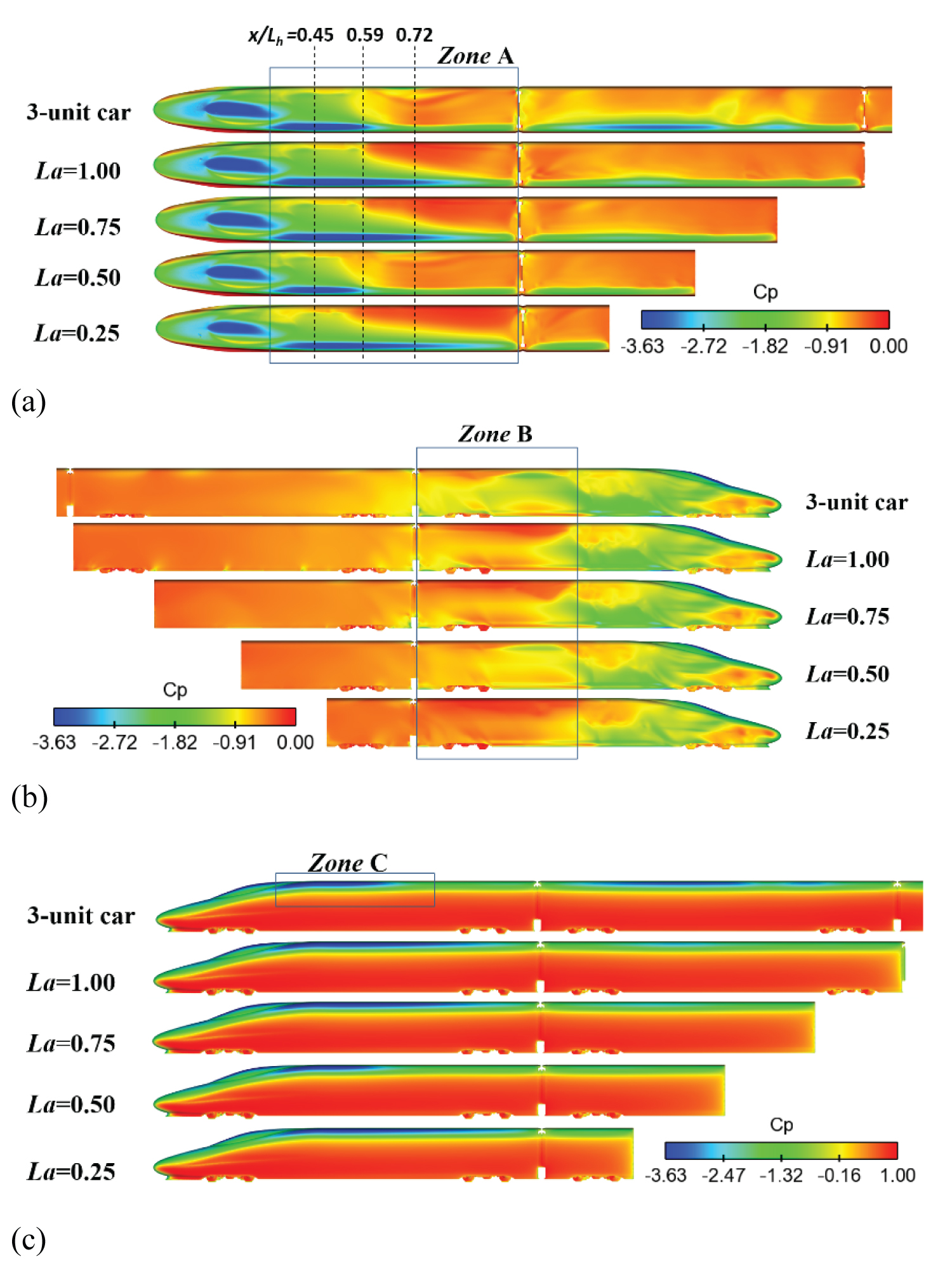
Figure 13 presents the pressure contours on train surface for different scenarios. It can be seen in Figure 13a that roof side is mainly negative pressure, and the negative zone A is reduced along with the lengthwise. At the slice location of x/L_h = 0.59, the strong negative regions at roof transition are weaker for L^a = 3-uint car and 0.50, and this is also reflected in Figure 10b of the pressure change curves. In addition, the negative pressure becomes steady and average both for L^a = 3-uint car and 0.50 whilst there are distinct pressure gradations for the rest cases. On the leeward side in Figure 13b, the apparent discrepancies occurred at zone B were smaller and even negative pressure distribution for L^a = 0.50 and L^a = 3-uint car. However, the obvious pressure layers are observed for L^a = 0.75 and L^a = 1.00 at zone B. For 3-uint cars, the pressure distribution at zone B is relatively large and average. On the windward side for different L^a lengths in Figure 13c, there is mainly positive pressure due to the stagnation of the incoming flow, with the largest discrepancy at the transition zone C where the flow crosses over and separates at the roof from the windward side. These phenomena indicate that downstream body length indeed affects flow patterns around the head car, leading to similar or different pressure distributions of the head car at different zones.

Flow field analysis around the train (β = 60°)

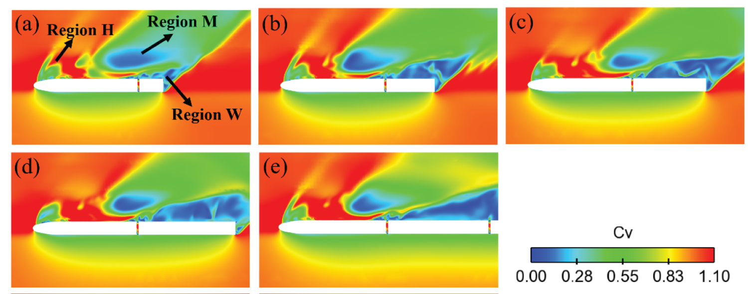
As the discrepancies in the pressure distribution are normally caused by the airflow around the train. It is necessary to analyze the flow structures around the head car to better understand the mechanism that makes these differences described above Figure 14 shows the velocity contours at z = 1.0 m for trains with different downstream body lengths. It is revealed in Figure 14 that the turbulent wake region W attached at leeward of the dummy body differs obviously. The flow of region W separates from the inter-carriage windshield to the end of the dummy body under the yaw effects. The wake flow region W develops and enlarged from L^a = 0.25 up to L^a = 1.00. While for a 3-unit car, due to the longer length of the downstream vehicle, the flow separates up to the tail car, resulting in the region W being quite steady and average compared with other cases.

Note there is a low velocity region M with a large scope at the leeward side of the head car, and the range of region M decreases from L^a= 0.25 up to L^a= 1.00. For shorter L^a length, such as L^a= 0.25, the wake region W affects the region M due to their closer distance. As the downstream body length increases, the turbulent wake flow moves downward, this influence becomes dim. As for Region H at the leeward of the streamlined head, the flow separates once crosses over the nose region, leading to a low velocity Region H. The shape types of Region H can be roughly divided into two categories: one is the L^a= 0.25, 0.50, and 3-uint car with extra branch, and another is L^a= 0.75, 1.00 without extra branch. The difference of Region H is mainly caused by the location change of Region M. When the vortex core of Region M is located upstream of the first windshield (i.e. L^a= 0.25, 0.50, and 3-unit car), the nose region H is more affected by region M due to their closer distance. When the vortex core of Region M is located in the middle of the first windshield (i.e. L^a= 0.75, 1.00), the nose region H is less influenced, thus no branch flow has occurred. In summary, at a large yaw angle, the downstream wake region W would directly affect the location of the low-velocity region M, furthermore the region M then would affect the upstream Region H accordingly.

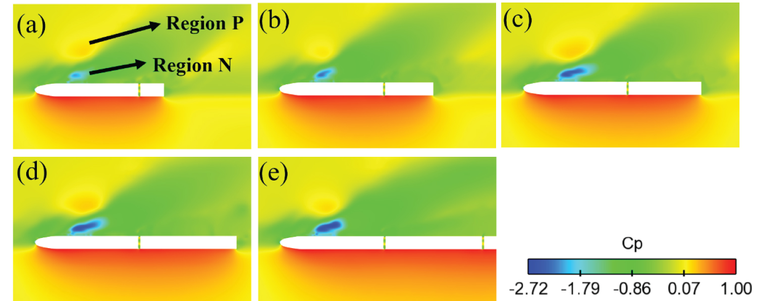
Figure 15 depicts the static pressure contours at the same location of Figure 14. It is observed in Figure 15 that a negative Region N is formed at the end of the streamlined head on the leeward. Additionally, a strong positive region P is observed nearly at the same location but away from the train body. With the increase of the downstream body length, the negative Region N gradually develops. This phenomenon indicates that shorter downstream body length contributes to pressure alleviation of the strong negative region N. For positive Region P, however, the range becomes smaller from L^a= 0.25 to L^a = 0.50 but increases again for L^a = 0.75 and L^a = 1.00.

In order to deeply analyze the airflow around the trains with different ends, the flow streamlines in terms of mean velocity coefficient at cut-plane x/L_h= 0.59 are drawn in Figure 16. An obvious small vortex V₁ can be found at the bottom of the subgrade, and there is no evident discrepancy of V₁ for various downstream vehicle lengths. When the airflow is impeded by the car body, the airflow will climb and cross over the roof, separating at certain locations. A small vortex V₂ is detected at the point where flow separation occurs. Note that the flow separates at the roof for cases L^a = 0.50 and 3-unit car while the airflow clinging to the roof and separates at the corner for the rest cases. This phenomenon results in different vortex sizes of V₂ and changes in the loads acting on the train roof, leading to similar aerodynamic lift force coefficients between L^a= 0.5 and 3-unit cars. Apart from V₂, another large vortex V₃ occurs at the leeward side, whose vortex core is away from the train body. For shorter downstream body lengths, such as L^a = 0.25, 0.50, the velocity is quite lower while the velocity of the vortex core increases for longer lengths.

Summary

The aerodynamic characteristics of trains with different downstream body lengths are numerically investigated. The aerodynamic coefficients and the flow field around the lead car are performed using the IDDES method combined with the Shear-Stress-Transport (SST) k-ω turbulence model. Train models with five different downstream body lengths are proposed to represent typical cases in the wind tunnel at the yaw angle ranging from 0° to 60°. The downstream dummy body length has the greatest effects on aerodynamic coefficients at high yaw angle (β > 30°), especially at β = 60°, where the flow pattern is detached-dominant, whereas the effects become insignificant at low yaw angle (β < 30°). For various downstream body lengths, the notable discrepancies appear at leeward and roof where large vortex shedding off. The larger contributions to the lateral force and lift force coefficients are mainly due to these areas. The aerodynamic behaviors and flow patterns of the downstream length of L^a = 0.50 and 3-unit car are highly relevant, both in aerodynamic force coefficients, surface pressure distribution and flow structures. The length of the downstream body affects the range and intensity of the wake flow, and this will have an associated impact on the vortex location on the leeward side, and finally, the distance of the vortex cores will in turn influence the flow field at nose region.

Funding

This work was supported by the National Railway Administration of China (Grant No. 18T043; No. 2018Z035) and the Fundamental Research Funds for Central South University Central Universities (Grant No. 2021zzts0170).

References

1. Gallagher M, Morden J, Baker C, et al. (2018) Trains in crosswinds–comparison of full-scale on-train measurements, physical model tests and CFD calculations. Journal of Wind Engineering and Industrial Aerodynamics 175: 428-444.
2. Hamidi H, Baker C (2010) L^arge-eddy simulation of the flow around a freight wagon subjected to a crosswind. Computers & Fluids 39: 1944-1956.
3. Morden, JA, Hemida H, Baker C (2015) Comparison of RANS and detached eddy simulation results to wind-tunnel data for the surface pressures upon a class 43 high-speed train. Journal of Fluids Engineering 137.
4. Bocciolone M, Cheli F, Corradi R, et al. (2008) Crosswind action on rail vehicles: Wind tunnel experimental analyses. Journal of Wind Engineering and Industrial Aerodynamics 96: 584-610.
5. Cheli F, Corradi R, Rocchi D, et al. (2010) Wind tunnel tests on train scale models to investigate the effect of infrastructure scenario. Journal of Wind Engineering and Industrial Aerodynamics 98: 353-362.
6. Niu J, Liang X, Zhou D (2016) Experimental study on the effect of Reynolds number on aerodynamic performance of high-speed train with and without yaw angle. Journal of Wind Engineering and Industrial Aerodynamics 157: 36-46.
7. Zhang L, Yang, MZ, Liang XF (2018) Experimental study on the effect of wind angles on pressure distribution of train streamlined zone and train aerodynamic forces. Journal of Wind Engineering and Industrial Aerodynamics 174: 330-343.
8. BS EN (2010) Railway applications–aerodynamics part 6: requirements and test procedures for cross wind assessment. London: British Standard Institute 14067-6.
9. Bell JR, Burton D, Thompson MC, et al. (2017) The effect of tail geometry on the slipstream and unsteady wake structure of high-speed trains. Experimental Thermal and Fluid Science 83: 215-230.
10. Schober M, Siefkes T Tengstrand H (2010) Two Years of Success–Bombardier’s Formula for Total Train Performance, 2010.
11. Dorigatti F, Sterling M, Baker CJ (2015) Crosswind effects on the stability of a model passenger train: A comparison of static and moving experiments. Journal of Wind Engineering and Industrial Aerodynamics 138: 36-51.
12. Zhang J, He K, Wang J (2019) Numerical simulation of flow around a high-speed train subjected to different windbreak walls and yaw angles. Journal of Applied Fluid Mechanics 12: 1137-1149.
13. Premoli A, Rocchi D, Schito P (2016) Comparison between steady and moving railway vehicles subjected to crosswind by CFD analysis. Journal of Wind Engineering and Industrial Aerodynamics 156: 29-40.
14. Cheli F, Ripamonti F, Rocchi D (2010) Aerodynamic behaviour investigation of the new EMUV₂50 train to cross wind. Journal of Wind Engineering and Industrial Aerodynamics 98: 189-201.
15. ANSYS (2016) Inc. ANSYS Fluent User’s Guide, Release.
16. Eichinger, Sándor, Mikael Sima (2015) Numerical simulation of a regional train in crosswind. Proceedings of the Institution of Mechanical Engineers. Part F: Journal of Rail and Rapid Transit 229: 625-634.
17. Flynn D, Hemida H, Baker C (2016) On the effect of crosswinds on the slipstream of a freight train and associated effects. Journal of Wind Engineering and Industrial Aerodynamics 156: 14-28.
18. Sakuma Y, Ido A (2009) Wind tunnel experiments on reducing separated flow region around front ends of vehicles on meter-gauge railway lines. Quarterly Report of RTRI 50: 20-25.
19. Ishak IA, Mat Ali MS Mohd, Yakub MF (2019) Effect of crosswinds on aerodynamic characteristics around a generic train model. International Journal of Rail Transportation 7: 23-54.
20. Chen Z, Liu T, Jiang Z (2018) Comparative analysis of the effect of different nose lengths on train aerodynamic performance under crosswind. Journal of Fluids and Structures 78: 69-85.
21. Chen JW, Gao GJ, Zhu CL (2016) Detached-eddy simulation of flow around high-speed train on a bridge under cross winds. Journal of Central South University 23: 2735-2746.
22. Miao XJ, Gao GJ (2015) Influence of ribs on train aerodynamic performances. Journal of Central South University 22: 1986-1993.