Dielectric Materials with Memory I: Minimum and General Free Energies

Abstract

A general tensor isothermal theory of free energies and free enthalpies for dielectrics is presented, corresponding to linear constitutive relations with memory. Starting from the general equations of continuum thermodynamics, various properties of and constraints on free energy/enthalpy functionals in dielectric media are noted. It is well-known that free enthalpies are particularly convenient in that their properties are closely analogous with those of free energies in mechanics, though different in crucial ways.

General constitutive equations with memory are determined from a given free enthalpy. The form of the relaxation function, which occurs in these constitutive equations, is discussed from a general viewpoint. Also, various forms of the work function are given.

Tensor formulae are derived for the minimum free energy and corresponding rate of dissipation for arbitrary and also sinusoidal histories of the electric and magnetic fields. Both the similarities with mechanics and the important differences, leading to different physical predictions, are emphasized throughout this work.

Introduction

Materials subject to electromagnetic fields or mechanical deformation processes, with constitutive equations involving memory effects, necessarily exhibit energy dissipation, so that thermo dynamical concepts [1-4] are required to describe their behavior.

It has been known for several decades that the free energy of a material with memory is not in general uniquely determined by the constitutive equations (for example [5-14,18-22,27-30,33]). For a given free energy, the total dissipation in the material over a given time period and the rate of dissipation are not uniquely determined either.

It can be shown in a very general context ([5,6] and later references [7-10], which are based on the earlier work) that the free energies corresponding to a given state of a physical (electromagnetic or viscoelastic, for example) system form a convex set, which is bounded and thus has a maximum and minimum value. The minimum free energy of a given state is equal to the maximum amount of work that can be recovered from that state. The maximum free energy of a state is equal to the minimum amount of work required to achieve that state.

An expression for the minimum free energy of a material with a linear memory-dependent constitutive equation was given for the scalar case in [11], in the context of mechanics and related to linear viscoelastic materials. This method was adapted to a dielectric material with memory in [12]. A generalization of [11] to tensor constitutive equations was given in [13]. This approach was developed over the last fifteen years to give explicit forms for the minimum, maximum and a family of intermediate free energies, mainly in a mechanics context. Most of these papers were based explicitly on a foundation of non-equilibrium thermodynamics of materials with memory, as developed in [1-4], and referred to as Rational Thermodynamics.

Indeed, thermodynamical concepts and language are explicitly used throughout the present work. In particular, constraints which are consequences of the laws of thermodynamics are presented and their physical consequences explored. We discuss the minimum free energy in a manner which generalizes [12] and also [14]. Tensor formulae are derived for this and related quantities of interest. An expression for the minimum free energy in the case of sinusoidal histories is derived for a general material.

The developments in this work are similar to the corresponding theory for mechanics and heat flow, described in [10] and references therein. These similarities are rendered clear by means of references to the relevant mechanics literature, usually [10]. However, there are various important differences and the exploration of these is at the core of what is new about the present work. The major difference derives from the formula (3.2) for the rate of work done on the material, which differs from the mechanics formula. This leads to important physical differences in material behavior, but also in the mathematical description of these materials.

This paper constitutes part I of a two part work, the remainder being referred to as part II. A new family of free energies is derived in the latter paper.

Some results in this context were given independently [15-17] for dielectric materials with memory, but with quite different methods, notation and terminology. These papers emerged out of ongoing work over a decade or so, exploring various physical issues in optics, quite distant from the continuum thermodynamics environment which generated the papers referred to in the above paragraphs.

We seek to bring these two streams together; in particular, the correspondence between the two terminologies is clarified.

The work discussed above refers to free energies derived from extremum conditions (minimum, maximum etc). Other functionals which are free energies only for materials with kernels obeying monotonicity conditions are discussed in [14,18,19] for example. With one exception [18], these emerge from the older literature. They are less relevant for dielectrics than in mechanics, in that the required monotonicity restrictions may not so frequently apply.

On the matter of notation, vectors and tensors are denoted by lowercase and uppercase boldface characters respectively and scalars by ordinary script. The real line is denoted by $\mathcal{R}$, the non-negative reals by ${\mathcal{R}}^{+}$ and the strictly positive reals by ${\mathcal{R}}^{+}{}^{+}$. Similarly, $\mathcal{R}{-}^{}$ is the set of non-positive reals and $\mathcal{R}{-}^{}{}^{-}$ the strictly negative reals. We will be dealing with spaces of scalar quantities with values in $\mathcal{R}$ or ${\mathcal{R}}^{+}$, vector quantities in ${\mathcal{R}}^3$ and second order tensors. Let one of these spaces, or a composite of more than one (for example ${\mathcal{R}}^3\times {\mathcal{R}}^3$), be denoted by $\mathcal{V}$. The space of linear operators $\mathcal{V}\mapsto \mathcal{V}$ is denoted by $Lin\left(\mathcal{V}\right)$. The dot product will indicate an ordinary scalar product ${\mathcal{R}}^3\times {\mathcal{R}}^3\mapsto \mathcal{R}$ and ${\mathcal{R}}^6\times {\mathcal{R}}^6\mapsto \mathcal{R}$.

Complex quantities arise in the frequency domain so we have complex vector spaces for which the dot product involves using the complex conjugate of objects in the dual space. The magnitude squared, denoted by ${|.|}^2$ refers to the dot product of objects with their complex conjugates.

General Relations

Consider a rigid dielectric material, subject to a varying electromagnetic field. Let the body under consideration occupy a volume $\mathcal{B}\subset {\mathcal{R}}^3$. A typical point in $\mathcal{B}$ is x while t is a given time. The electric field on this region is E(x,t), with electric displacement denoted by D(x,t). The magnetic field is H(x,t) and the magnetic induction B(x,t). Let us introduce a convenient compact notation [12]. The quantities $\Lambda \text{ : }{\mathcal{R}}^3\times \mathcal{R}\mapsto {\mathcal{R}}^6$ and $\sum \text{ : }{\mathcal{R}}^3\times \mathcal{R}\mapsto {\mathcal{R}}^6$, respectively the electromagnetic vector and the electromagnetic induction, are defined by

$$\Lambda \text{ = (}{\rm E}\text{, }{\rm H}\text{), }\sum \text{ = (}D\text{, }B\text{)}\text{. (3}\text{.1)}$$

We shall denote ${\mathcal{R}}^6$ by $\mathcal{V}$ in what follows for a slight gain in brevity but also to emphasize that the general developments apply to an arbitrary finite vector space. The quantity $\Lambda$ will be treated as the independent variable. We will generally omit the space variable x and sometimes t also. It is assumed that $\Lambda \left(s\right)$, $s\text{ < }t$ is continuously differentiable with respect to time. The rate of work done by the electromagnetic field on the body, per unit volume, is ([14] and references therein)

$$p\text{ = }\dot{\sum }\cdot \Lambda \text{ = }{\dot{\sum }}^T\Lambda ,(3.2)$$

Where the dot product here represents a scalar product in $\mathcal{V}$ and ${\dot{\sum }}^T$ is the transpose of $\dot{\sum }$. Of these two alternative notations, the first will be used in the present work, as in previous related papers on similar problems in mechanics. The internal energy per unit mass and the entropy per unit mass at (x,t), both scalar quantities, are denoted respectively by $\in \left(x,t\right)$ and $\eta \left(x,t\right)$. The local absolute temperature is $\theta \left(x,t\right)\in {\mathcal{R}}^{+}$. The heat flux vector is $q\left(x,t\right)\in {\mathcal{R}}^3$.

The energy balance equation or first law of thermodynamics has the form

$$p-\rho \dot{\in }-\nabla \cdot q+\rho r\text{ = 0, (3}\text{.3)}$$

Where p is defined by (3.2) and the differential operator $\nabla$ is with respect to x. The quantity $\rho \left(x\right)$ is the mass density, which can depend on position but not time and $r\left(x,t\right)$ is the external heat supply absorbed per unit time, per unit mass at (x,t). We write the second law of thermodynamics as

$$\dot{\eta }\text{+}\frac{1}{\rho }\nabla \cdot \left(\frac{q}{\theta }\right)\ge \frac{r}{\theta }.\text{ (3}\text{.4)}$$

Which is a statement that the rate of entropy production is non-negative. The superimposed dot notation in (3.3) - (3.4) and below, indicates a time derivative.

Remark Ⅲ.1

Equations (3.3), (3.4) are generalizations to electromagnetic fields of the classical laws of thermodynamics. If we neglect r and integrate (3.3) over a volume large enough so that no heat is passing through the boundary, the term involving q vanishes by Green's theorem, and the other terms yield a simple statement of conservation of energy for a finite body subject to electromagnetic forces.

The Helmholtz free energy per unit mass is defined by

$$\psi \text{ = }\in -\theta \eta .\text{ (3}\text{.5)}$$

with the aid of (3.5) and a simple identity, (3.3) can be rewritten in the form

$$\frac{p}{\rho }-\dot{\psi }-\eta \dot{\theta }-\frac{1}{\rho \theta }(\nabla \theta )\cdot q\text{ = }D,(3.6)$$

$$D\text{ = }\theta \dot{\eta }\text{+}\frac{\theta }{\rho }\nabla \cdot \left(\frac{q}{\theta }\right)-r\ge \text{0,}$$

Where, in the second relation, we have invoked (3.4).

Let us now consider the isothermal case where $\theta$ is independent of space and time variables, q is zero and r is assumed to be negligible. Also, we take $\rho$ to be constant and put it equal to unity. Thus, (3.6) becomes

$$\dot{\psi }\text{+ }D\text{ = }\dot{\sum }\cdot \Lambda (3.7\text{a})$$

$$D\text{ = }\dot{\eta }\theta .\text{ (3}\text{.7b)}$$

The second law is imposed through the requirement that

$$D\text{ = }\dot{\sum }\cdot \Lambda -\dot{\psi }\ge \text{0}\text{. (3}\text{.8)}$$

Remark Ⅲ.2

In a mechanics context, the time differentiation in (3.7) would be on the $\Lambda$, corresponding to the strain tensor, rather than on the $\sum$, corresponding to the stress tensor. Thus, the theory developed here is analogous to the case in mechanics where the stress is treated as the independent variable and, as we shall see, the memory functions involved will behave similarly to creep rather than relaxation functions, in the sense that they tend to increase rather than decrease with time.

Let ${\Lambda }^t\text{ : }{R}^{+}\mapsto \mathcal{V}$ be defined by^a

$${\Lambda }^t(s)\text{ = }\Lambda \text{(}t-s),s\in {\mathcal{R}}^{+}.\text{ (3}\text{.9)}$$

We assume that these belong to a real Hilbert space $\mathcal{H}$ of functions with values in $\mathcal{V}$, possessing a suitable inner product and norm. The norm is understood to have a fading memory property, in the sense that values of field quantities at times in the distant past contribute negligibly to its value. Equation (3.9) gives the history and current value of $\Lambda$. A given future continuation is denoted by

$${\Lambda }^t(s)\text{ = }\Lambda \text{(}t-s),s\in {\mathcal{R}}^{--}.\text{ (3}\text{.10)}$$

Let us define the free enthalpy as

$$\mathcal{F}\text{ = }\psi -\sum \cdot \Lambda ,(3.11)$$

which is analogous to the Gibbs free energy in mechanics. The quantity $\sum \cdot \Lambda$ is of course unique, so that to each free energy, there is a corresponding free enthalpy. In terms of this quantity, (3.7) and (3.8) become

$$\dot{\mathcal{F}}\text{+}D\text{ = }-\sum \cdot \dot{\Lambda }(3.12\text{a})$$

$$D\ge 0\text{ (3}\text{.12b)}$$

the latter being the second law. A constitutive assumption is now made by requiring that the free enthalpy $\mathcal{F}$ depends in a specified way on the history and current value of $\Lambda$. We put^b

$$\mathcal{F}(t)\text{ = }\underset{s>0}{\overset{\sim }{\mathcal{F}}}\left({\Lambda }^t(s),\Lambda (t)\right).\text{ (3}\text{.13)}$$

Details and more general insights of the developments now briefly summarized may be found in [1-4]. Assuming that $\tilde{\mathcal{F}}$ is differentiable with respect to $\Lambda (t)$ and Fréchet-differentiable with respect to ${\Lambda }^t$ within $\mathcal{H}$, we can apply the chain rule to obtain

$$\begin{array}{l}\frac{d}{dt}\underset{s>0}{\overset{\sim }{\mathcal{F}}}\left({\Lambda }^t(s),\Lambda (t)\right)\text{ = }{\partial }_{\Lambda (t)}\underset{s>0}{\overset{\sim }{\mathcal{F}}}\left({\Lambda }^t(s),\Lambda (t)\right)\cdot \dot{\Lambda },(3.14)\\ +\delta \underset{s>0}{\overset{\sim }{\mathcal{F}}}\left({\Lambda }^t(s),\Lambda (t)|\frac{\partial }{\partial t}{\Lambda }^t(s)\right)\end{array}$$

where ${\partial }_{\Lambda \left(t\right)}$ indicates the derivative of $\tilde{\mathcal{F}}$ with respect to the current value $\Lambda (t)$ and $\delta \tilde{\mathcal{F}}$ is the Fréchet-differential of $\tilde{\mathcal{F}}$ at ${\Lambda }^t$ in the direction $\frac{\partial }{\partial t}{\Lambda }^t$ where, from (3.9),

$$\frac{\partial }{\partial t}{\Lambda }^t(s)\text{ = }-\frac{\partial }{\partial s}{\Lambda }^t(s).\text{ (3}\text{.15)}$$

These derivatives with respect to field quantities are assumed to be continuous in their arguments. Within the context of Rational Thermodynamics, it can be shown that $\dot{\Lambda }(t)$ may be chosen to have any desired value, so that it follows from (3.14), combined with (3.12b), that

$$\sum (t)\text{ = }-{\partial }_{\Lambda (t)}\underset{s>0}{\overset{\sim }{\mathcal{F}}}\left({\Lambda }^t(s),\Lambda (t)\right),\text{ (3}\text{.16)}$$

which are the constitutive equations of the material; also,

$$D(t)\text{ = }-\delta \underset{s>0}{\overset{\sim }{\mathcal{F}}}\left({\Lambda }^t(s),\Lambda (t)|\frac{\partial }{\partial t}{\Lambda }^t(s)\right).\text{ (3}\text{.17)}$$

Thus, we see that dissipation in the material is associated with the dependence of $\mathcal{F}$ and $\psi$ on the past history of the field variables (including limiting cases such as a dependence on time derivatives of these variables). If no such dependence on past values of field variables exists, the rate of dissipation is zero.

We can also write (3.13) in the form

$$\mathcal{F}(t)\text{ = }\underset{s>0}{\overset{\sim }{{\mathcal{F}}_d}}\left({\Lambda }_r^t(s),\Lambda (t)\right),\text{ (3}\text{.18)}$$

where the relative history ${\Lambda }_r^t$ is defined by

$${\Lambda }_r^t(s)\text{ = }{\Lambda }^t(s)-\Lambda (t).\text{ (3}\text{.19)}$$

A relative future continuation is also defined by (3.19) for $s\in {\mathcal{R}}^{--}$.

We define the equilibrium free enthalpy ${\mathcal{F}}_e(t)$ to be given by (3.13) for the static history ${\Lambda }^t(s)-\Lambda (t)$, $s\in {\mathcal{R}}^{+}$ or equivalently by (3.18) with ${\Lambda }_r^t(s)\text{ = 0}$, $s\in {\mathcal{R}}^{+}$. This quantity depends only on $\Lambda (t)$, so that

$${\mathcal{F}}_e(t)\text{ = }{\tilde{\mathcal{F}}}_e(\Lambda (t)).\text{ (3}\text{.20)}$$

It can be deduced from (3.12), by means of a fading memory argument [3], that

$${\mathcal{F}}_e(t)\le \mathcal{F}(t),\forall t\in \mathcal{R}\text{ , (3}\text{.21)}$$

giving that the equilibrium free enthalpy is less than or equal to the free enthalpy for an arbitrary history. The notation ${\mathcal{F}}_e(t)$ will be used in most cases rather than ${\tilde{\mathcal{F}}}_e(\Lambda (t))$.

We can write (3.18) in the form

$$\mathcal{F}(t)\text{ = }{\mathcal{F}}_e(t)+{\tilde{\mathcal{F}}}_M\left({\Lambda }_r^t(s),\Lambda (t)\right),\text{ (3}\text{.22)}$$

where the second term on the right must be non-negative by virtue of (3.21). It contains the memory contributions.

Required properties of a free enthalpy

Let us state the characteristic properties of a free enthalpy, provable within a general framework [3,4,12]:

P1:

$$\frac{\partial \mathcal{F}(t)}{\partial \Lambda (t)}\text{ = }-\sum (t),\text{ (3}\text{.23)}$$

which is (3.16).

P2:

For any history ${\Lambda }_a^t$ and current value ${\Lambda }_a(t)$,

$$\tilde{\mathcal{F}}({\Lambda }_a^t,{\Lambda }_a(t))\ge {\tilde{\mathcal{F}}}_e({\Lambda }_a(t)),\text{ (3}\text{.24)}$$

which is (3.21).

P3:

Condition (3.12) holds.

These will be referred to as the Graffi conditions by analogy with those for a free energy in mechanics (for example [10], page 115).

Remark Ⅲ.3:

For materials with memory, there are in general an infinity of choices of $\mathcal{F}$ (and the corresponding $\psi$ given by (3.11)) that have the required properties. Each of these has a corresponding rate of dissipation D, obeying (3.7a). These are different versions of the first law, one of which is the correct version, giving the physically observed rate of dissipation. The others can be seen as approximations and in some cases bounds on the physical quantities. A proposed physical free energy is presented in [20,21]. The general question of how to determine the physical rate of dissipation is discussed in [10], page 131 and [22].

A Linear Memory Model

We expand (3.22) to second order in a functional Taylor expansion, dropping the linear term because of positivity requirements and also neglecting higher order terms [21], to obtain

$$\mathcal{F}\left(t\right)\text{ = }{\mathcal{F}}_e\left(t\right)\text{+}\frac{1}{2}{\displaystyle {\int }_0^{\infty }{\displaystyle {\int }_0^{\infty }{\Lambda }_r^t}}\left(s\right)\cdot \mathbb{K}\left(s,u\right){\Lambda }_r^t\left(u\right)dsdu,\text{ (4}\text{.1)}$$

Where $\mathbb{K}\text{ : }{\mathcal{R}}^{+}\text{ x }{\mathcal{R}}^{+}\mapsto Lin\left(\mathcal{V}\right)$ can be taken to obey the relation

$${\mathbb{K}}^T\left(s,u\right)\text{ = }\mathbb{K}\left(u,s\right),\text{ (4}\text{.2)}$$

without loss of generality. A dependence in the kernel $\mathbb{K}$ on $\Lambda (t)$ has also been neglected [21].

Remark Ⅳ.1:

The integral term in (4.1) must be non-negative by virtue of (3.24). By considering much localized histories, we can see that a necessary condition for this property to hold is that

$$\mathbb{K}\left(s,s\right)\ge 0,s\in {\mathcal{R}}^{+},\text{ (4}\text{.3)}$$

which corresponds to the condition on diagonal components in non-negative matrices.

Remark Ⅳ.2:

The integral in (4.1) is a quadratic functional of tensor quantities, which can be expressed as sums of scalar quadratic functionals by using appropriate eigenspaces [10].

Quadratic functionals of this kind are the simplest forms which include memory effects and on which we can impose a positivity requirement. Such a requirement is essential for energy related quantities, including, because of the second law, dissipation. These observations are also relevant to (4.15) and (4.23) below.

We shall see below that such a quadratic functional for the free enthalpy leads to linear constitutive relations for the material. Let us define $\mathbb{L}\text{ : }{\mathcal{R}}^{+}\text{ x }{\mathcal{R}}^F+\mapsto Lin\left(\mathcal{V}\right)$ by

$$\mathbb{L}\left(s,u\right)\text{ = }{\mathbb{L}}_{\infty }-{\displaystyle \underset{s}{\overset{\infty }{\int }}{\displaystyle \underset{u}{\overset{\infty }{\int }}\mathbb{K}\left(t_{1,}{t}_2\right)}}d{t}_{1}d{t}_2,\text{ (4}\text{.4)}$$

where ${\mathbb{L}}_{\infty }$ is a constant tensor in $Lin\left(\mathcal{V}\right)$, to be determined, but assumed to be symmetric so that

$${\mathbb{L}}_{\infty }\text{ = }{\mathbb{L}}_{\infty }^T\text{ (4}\text{.5)}$$

It follows that

$$\frac{{\partial }^2}{\partial s\partial u}\mathbb{L}\left(s,u\right)\text{ = }{\mathbb{L}}_{12}\left(s,u\right)\text{ = }-\mathbb{K}\left(s,u\right),\text{ (4}\text{.6a)}$$

$$\underset{s\to \infty }{\lim }\mathbb{L}\left(s,u\right)\text{ = }{\mathbb{L}}_{\infty },u\in {\mathcal{R}}^{+},\text{ (4}\text{.6b)}$$

$$\underset{s\to \infty }{\lim }\frac{\partial }{\partial u}\mathbb{L}\left(s,u\right)\text{ = 0},u\in {\mathcal{R}}^{+},\text{ (4}\text{.6c)}$$

$$\underset{s\to \infty }{\lim }\frac{\partial }{\partial s}\mathbb{L}\left(s,u\right)\text{ = 0},u\in {\mathcal{R}}^{+},\text{ (4}\text{.6d)}$$

$${\mathbb{L}}^T\left(s,u\right)\text{ = }\mathbb{L}\left(u,s\right),\text{ (4}\text{.6e)}$$

with similar limits at large u holding for fixed s. Using relevant relations from (4.6) and partial integrations, we can write (4.1) as

$$F\left(t\right)\text{ = }{\mathcal{F}}_e\left(t\right)-\frac{1}{2}{\displaystyle {\int }_0^{\infty }{\displaystyle {\int }_0^{\infty }{\Lambda }_r^t}}\left(s\right)\cdot {\mathbb{L}}_{12}\left(s,u\right){\Lambda }_r^t\left(u\right)dsdu,\text{ (4}\text{.7a)}$$

$$\text{= }{\mathcal{F}}_e\left(t\right)-\frac{1}{2}{\displaystyle {\int }_0^{\infty }{\displaystyle {\int }_0^{\infty }{\stackrel{·}{\Lambda }}^t}}\left(s\right)\cdot \tilde{\mathbb{L}}\left(s,u\right){\stackrel{·}{\Lambda }}^t\left(u\right)dsdu,\text{ (4}\text{.7b)}$$

Where

$${\stackrel{·}{\Lambda }}^t\left(u\right)\text{ = }\frac{\partial }{\partial t}{\Lambda }^t\left(u\right)\text{ = }-\frac{\partial }{\partial u}{\Lambda }^t\left(u\right)\text{ = }-\frac{\partial }{\partial u}{\Lambda }_r^t\left(u\right),\text{ (4}\text{.8a)}$$

$$\tilde{\mathbb{L}}\left(s,u\right)\text{ = }\mathbb{L}\left(s,u\right)-{\mathbb{L}}_{\infty }.\text{ (4}\text{.8b)}$$

Relation (3.23) gives

$$\sum \left(t\right)\text{ = }{\tilde{\sum }}_e\left(\Lambda \left(t\right)\right)\text{+}{\displaystyle {\int }_0^{\infty }{\mathbb{L}}^{\prime }}\left(u\right){\Lambda }_r^t\left(u\right)du,\text{ (4}\text{.9a)}$$

$$={\sum }_0\left(t\right)\text{+}{\displaystyle {\int }_0^{\infty }{\mathbb{L}}^{\prime }}\left(u\right){\Lambda }^t\left(u\right)du,\text{ (4}\text{.9b)}$$

$$={\tilde{\sum }}_e\left(\Lambda \left(t\right)\right)\text{+}{\displaystyle {\int }_0^{\infty }\tilde{\mathbb{L}}}\left(u\right){\stackrel{·}{\Lambda }}^t\left(u\right)du,\text{ (4}\text{.9c)}$$

Where

$$\mathbb{L}\left(u\right)\text{ = }\mathbb{L}\left(0,u\right),\text{ (4}\text{.10a)}$$

$${\mathbb{L}}_0\text{ = }\mathbb{L}\left(0,\text{0}\right)\text{ = }\mathbb{L}\left(0\right),\text{ (4}\text{.10b)}$$

$$\tilde{\mathbb{L}}\left(u\right)\text{ = }\mathbb{L}\left(u\right)-{\mathbb{L}}_{\infty },\text{ (4}\text{.10c)}$$

$${\mathbb{L}}^{\prime }\left(u\right)\text{ = }\frac{d}{du}\mathbb{L}\left(u\right),\text{ (4}\text{.10d)}$$

and

$${\tilde{\sum }}_e\left(\Lambda \left(t\right)\right)\text{ = }{\sum }_e\left(t\right)\text{ = }-\frac{d{\tilde{\mathcal{F}}}_e\left(\Lambda \left(t\right)\right)}{d\Lambda \left(t\right)},\text{ (4}\text{.11a)}$$

$${\sum }_0\left(t\right)\text{ = }{\tilde{\sum }}_e\left(\Lambda \left(t\right)\right)\text{ + }\left({\mathbb{L}}_0-{\mathbb{L}}_{\infty }\right)\Lambda \left(t\right).\text{ (4}\text{.11b)}$$

The quantity $\mathbb{L}\left(s\right)$ is the electromagnetic relaxation function. It is shown below (see (5.18)) that ${\mathbb{L}}_{\infty }$ is a positive definite matrix. The quantity $\mathbb{L}{0}_{}$ is the instantaneous modulus and, on the basis of physical evidence [12],

$${\mathbb{L}}_0>\text{ 0}\text{. (4}\text{.12)}$$

It will be assumed here, as in earlier work (in mechanics) on tensor constitutive relations [10], that

$$\mathbb{L}\left(u\right)\text{ = }{\mathbb{L}}^T\left(u\right),u\in {\mathcal{R}}^{+}.\text{ (4}\text{.13)}$$

By analogy with viscoelasticity, the quantity $\mathbb{L}{0}_{}$ is the instantaneous modulus, while ${\mathbb{L}}_{\infty }$ is the equilibrium modulus [12]. We are assuming that $\Lambda \left(-\infty \right)\text{ = }\Lambda t\left(\infty \right)$ vanishes. It follows from (4.6c) (though for large u rather than large s) and (4.10a) that

$${\mathbb{L}}_{\infty }\text{ = }\mathbb{L}\left(s,\infty \right)\text{ = }\mathbb{L}\left(0,\infty \right)\text{ = }\mathbb{L}\left(\infty \right).\text{ (4}\text{.14)}$$

We deduce from (3.12), (4.8) and the time derivative of (4.7b) that

$$D\left(t\right)\text{ = }\frac{1}{2}{\displaystyle {\int }_0^{\infty }{\displaystyle {\int }_0^{\infty }{\stackrel{·}{\Lambda }}^t}}\left(s\right)\cdot \left[{\mathbb{L}}_1\left(s,u\right)\text{ + }{\mathbb{L}}_2\left(s,u\right)\right]{\stackrel{·}{\Lambda }}^t\left(u\right)dsdu,\text{ (4}\text{.15)}$$

Where the subscripts indicate partial differentiation with respect to the first and second arguments, as in (4.6a). This expression results from two partial integrations. These manipulations are equivalent in this context to the functional differentiation involved in (3.17).After further partial integrations, using (4.8), the rate of dissipation can also be expressed as

$$D\left(t\right)\text{ = }\frac{1}{2}{\displaystyle {\int }_0^{\infty }{\displaystyle {\int }_0^{\infty }{\Lambda }_r^t}}\left(s\right)\cdot \left[{\mathbb{L}}_{112}\left(s,u\right)\text{+}{\mathbb{L}}_{212}\left(s,u\right)\right]{\Lambda }_r^t\left(u\right)dsdu.\text{ (4}\text{.16)}$$

Relation (4.9) allows for general nonlinear behavior in the equilibrium term ${\sum }_e$. We now however specialize to the case of linear behavior. Following [12,14], we write (4.9b) as

$$\sum \left(t\right)\text{ = }{\mathbb{L}}_0\Lambda \left(t\right)\text{ + }{\displaystyle {\int }_0^{\infty }{\mathbb{L}}^{\prime }}\left(u\right){\Lambda }^t\left(u\right)du,\text{ (4}\text{.17)}$$

So that, from (4.11b)

$${\sum }_e\left(t\right)\text{ = }{\mathbb{L}}_{\infty }\Lambda \left(t\right),\text{ (4}\text{.18)}$$

and equations (4.9a) and (4.9c) become

$$\sum \left(t\right)\text{ = }{\mathbb{L}}_{\infty }\Lambda \left(t\right)\text{+ }{\displaystyle {\int }_0^{\infty }{\mathbb{L}}^{\prime }}\left(u\right){\Lambda }_r^t\left(u\right)du\text{ (4}\text{.19a)}$$

$$={\displaystyle {\int }_0^{\infty }\mathbb{L}}\left(u\right){\stackrel{·}{\Lambda }}^t\left(u\right)du,\text{ (4}\text{.19b)}$$

Relation (4.19b) is analogous to the Boltzmann Superposition Principle in mechanics [23]. It follows from (4.11a) and (4.18) that

$${\mathcal{F}}_e\left(t\right)\text{ = }-\frac{1}{2}\Lambda \left(t\right)\cdot {\mathbb{L}}_{\infty }\Lambda \left(t\right),\text{ (4}\text{.20)}$$

provided we add the condition that ${\mathcal{F}}_e\left(t\right)$ must vanish when $\Lambda \left(t\right)\text{ = 0}$. Relation (4.7a) becomes

$$\mathcal{F}\left(t\right)\text{ = }-\frac{1}{2}\Lambda \left(t\right)\cdot {\mathbb{L}}_{\infty }\Lambda \left(t\right)-\frac{1}{2}{\displaystyle {\int }_0^{\infty }{\displaystyle {\int }_0^{\infty }{\Lambda }_r^t}}\left(s\right)\cdot {\mathbb{L}}_{12}\left(s,u\right){\Lambda }_r^t\left(u\right)dsdu\text{ (4}\text{.21a)}$$

$$\text{= }\frac{1}{2}\Lambda \left(t\right)\cdot {\mathbb{L}}_0\Lambda \left(t\right)-\sum \left(t\right)\cdot \Lambda \left(t\right)\text{ (4}\text{.21b)}$$

$$-\frac{1}{2}{\displaystyle {\int }_0^{\infty }{\displaystyle {\int }_0^{\infty }{\Lambda }^t}}\left(s\right)\cdot {\mathbb{L}}_{12}\left(s,u\right){\Lambda }^t\left(u\right)dsdu.$$

Since the integral term in (4.21b) is independent of $\Lambda \left(t\right)$, it follows that

$$\frac{\partial }{\partial \Lambda \left(t\right)}\left[\frac{1}{2}\Lambda \left(t\right)\cdot {\mathbb{L}}_0\Lambda \left(t\right)-\sum \left(t\right)\cdot \Lambda \left(t\right)\right]\text{ = }-\sum \left(t\right),\text{ (4}\text{.22)}$$

which is easily checked. From (3.11) and (4.21), we deduce that

$$\psi \left(t\right)\text{ = }{\varphi }_0\left(t\right)-\frac{1}{2}{\displaystyle {\int }_0^{\infty }{\displaystyle {\int }_0^{\infty }{\Lambda }^t}}\left(s\right)\cdot {\mathbb{L}}_{12}\left(s,u\right){\Lambda }^t\left(u\right)dsdu\text{ (4}\text{.23a)}$$

$$\text{= }U\left(t\right)-\frac{1}{2}{\displaystyle {\int }_0^{\infty }{\displaystyle {\int }_0^{\infty }{\Lambda }^t}}\left(s\right)\cdot {\mathbb{L}}_{12}\left(s,u\right){\Lambda }_r^t\left(u\right)dsdu,\text{ (4}\text{.23b)}$$

Where

$${\varphi }_0\left(t\right)\text{ = }\frac{1}{2}\Lambda \left(t\right)\cdot {\mathbb{L}}_0\Lambda \left(t\right),U\left(t\right)\text{ = }\sum \left(t\right)\cdot \Lambda \left(t\right)-\frac{1}{2}\Lambda \left(t\right)\cdot {\mathbb{L}}_{\infty }\Lambda \left(t\right).\text{ (4}\text{.24)}$$

The first term on the right of (4.23a) is non-negative by virtue of (4.12). This is not true of the first term on the right of (4.23b). From remark Ⅳ.1, we conclude that both integral terms, with the negative signs included, are non-negative.

It is of interest to compare the relations (4.23) with the corresponding expressions in mechanics ([10] page 127, for example). There are obvious important differences, but also more subtle ones, relating to the behavior of the kernel. In particular, the kernel of the constitutive relation (4.9), defined by (4.10a) is shown in subsection 5.1 to have different behavior from the corresponding quantity in mechanics.

From (3.2), it follows that the total work done by the electromagnetic field up to time t is

$$W\left(t\right)\text{ = }{\displaystyle {\int }_{-\infty }^t\sum ^{·}}\left(u\right)\cdot \Lambda \left(u\right)du\text{ (4}\text{.25a)}$$

$$=\sum \left(t\right)\cdot \Lambda \left(t\right)-{\displaystyle {\int }_{-\infty }^t\sum }\left(u\right)\cdot \stackrel{·}{\Lambda }\left(u\right)du.\text{ (4}\text{.25b)}$$

It is assumed here and below that field quantities vanish at large negative times sufficiently strongly so that various required integrals exist. Integrating (3.7a) on $(-\infty ,t\text{]}$, we have

$$\psi \left(t\right)\text{+}D\left(t\right)\text{ = }W\left(t\right),\text{ (4}\text{.26)}$$

Where

$$D\left(t\right)\text{ = }{\displaystyle {\int }_{-\infty }^{t}D\left(u\right)}du\ge \text{0, (4}\text{.27)}$$

is the total dissipation up to time t.

The physical content of (4.17) is hidden to some degree by the generality of the notation. It is worthwhile writing out in detail the relations implied by this expression. These are the most general within the category of an isothermal linear constitutive relation. We have

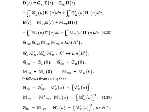
Examples of these relationships should be experimentally verifiable, supporting or otherwise the assumption (4.13).

Minimal states

Different histories may be members of the same minimal state. This is based on a concept of state originated by Giles and Noll [24,25], elaborated for the linear case in [9,13,26-28] and later work. The fundamental definition of the state of a material with memory at time t is the history of the independent field variable and its current value $\left({\Lambda }^t,\Lambda \left(t\right)\right)$. The concept of a minimal state is based on an equivalence class of states. Two states $\left({\Lambda }_1^t,{\Lambda }_1\left(t\right)\right),$,$\left({\Lambda }_2^t,{\Lambda }_2\left(t\right)\right)$ are equivalent, or in the same minimal state if from a time t onwards, we have

$${\sum }_1\left(t+s\right)\text{ = }{\sum }_2\left(t+s\right)\text{ if }{\Lambda }_1\left(t+s\right)\text{ = }{\Lambda }_2\left(t+s\right),s\ge \text{0 (4}\text{.30)}$$

Where ${\sum }_1,{\sum }_2$ are defined by (4.19) for these states. Note that the quantities in the second relation can be written as ${\Lambda }_1^t\left(-s\right)$ and ${\Lambda }_2^t\left(-s\right)$. It follows that

$${\displaystyle {\int }_0^{\infty }{\mathbb{L}}^{\prime }}\left(s+u\right)\left({\Lambda }_1^t\left(u\right)-{\Lambda }_2^t\left(u\right)\right)du\text{ = 0, }s\ge \text{0}\text{. (4}\text{.31)}$$

A fundamental distinction between materials is that for certain relaxation functions, namely those with only isolated singularities (in the frequency domain), the set of minimal states is non-singleton, while if some branch cuts are present in the relaxation function, the material has only singleton minimal states ([10,18], page 342). For relaxation functions with only isolated singularities, for example, sums of pole terms, there is a maximum free energy that is less than the work function $W\left(t\right)$ and also a range of related intermediate free energies. This case is explored for dielectrics in part II. On the other hand, if branch cuts are present, the maximum free energy is $W\left(t\right)$. An example of a branch cut would be if the relaxation function in the frequency domain (see (5.8) below) were an integral over pole terms, as for continuous spectrum materials in mechanics [29].

It can be shown that if the material has minimal states that are non-singleton then the free energy functional is positive semi-definite ([10], page 152).

Note that the statement that $\left({\Lambda }^t,\Lambda \left(t\right)\right)$ and $\left({\Lambda }_2^t,{\Lambda }_2\left(t\right)\right)$ are equivalent is the same as the assertion that $\left({\Lambda }_d^t,\text{ 0}\right)$ is equivalent to the zero state (0,0), where 0 is the zero in $\mathcal{V}$ (and also the zero history), while

$${\Lambda }_d^t\left(s\right)\text{ = }{\Lambda }_1^t\left(s\right)-{\Lambda }_2^t\left(s\right).\text{ (4}\text{.32)}$$

A functional of $\left({\Lambda }^t,\Lambda \left(t\right)\right)$ which yields the same value for all members of the same minimal state will be referred to as a functional of the minimal state or as a minimal state variable. Let $\left({\Lambda }_1^t,{\Lambda }_1\left(t\right)\right)$, $\left({\Lambda }_2^t,{\Lambda }_2\left(t\right)\right)$ be any equivalent states. Then, a free energy is a functional of the minimal state if

$$\psi \left({\Lambda }_1^t,{\Lambda }_1^t\left(t\right)\right)\text{ = }\psi \left({\Lambda }_2^t,{\Lambda }_2\left(t\right)\right).\text{ (4}\text{.33)}$$

It is not necessary that a free energy have this property, though it holds for the minimum and other free energies introduced in both parts of this work.

Kernels and Field Variables in the Frequency Domain

For any $f\in L^2\left(R\right)$, we denote its Fourier transform $f_F\in L^2\left(R\right)$ by^c

$$f_F\left(\omega \right)\text{ = }{\displaystyle {\int }_{-\infty }^{\infty }f\left(\xi \right)}{e}^{-i\omega \xi }d\xi \text{ = }{f}_{+}\left(\omega \right)+f_{-}\left(\omega \right),\text{ (5}\text{.1)}$$

$$f_{+}\left(\omega \right)\text{ = }{\displaystyle {\int }_0^{\infty }f\left(\xi \right)}{e}^{-i\omega \xi }d\xi ,f_{-}\left(\omega \right)\text{ = }{\displaystyle {\int }_{-\infty }^{\infty }f\left(\xi \right)}{e}^{-i\omega \xi }d\xi .$$

The quantities $f_{\pm }\left(\omega \right)$ are important in this work because of their analyticity properties noted in the paragraph before (5.20), among other reasons. For real valued functions in the time domain, we have

$${\overline{f}}_F\left(\omega \right)\text{ = }{f}_F\left(-\omega \right),\omega \in R,\text{ (5}\text{.2)}$$

where the bar denotes the complex conjugate. For complex values of $\omega$, (5.2) becomes

$$\overline{f_F\left(\omega \right)}\text{ = }{f}_F\left(-\overline{\omega }\right).\text{ (5}\text{.3)}$$

A time domain function defined on ${\mathcal{R}}^{+}$ is identified with a function on $\mathcal{R}$ which vanish identically on $\mathcal{R}{-}^{}{}^{-}$.In such cases,

$$f_F\left(\omega \right)=f_{+}\left(\omega \right)=f_c\left(\omega \right)-i{f}_s\left(\omega \right),\text{ (5}\text{.4)}$$

Where $f_c,f_s$ are respectively the Fourier cosine and sine transforms. Inverse transforms are given by

$$f\left(s\right)=\frac{1}{2\pi }{\displaystyle {\int }_{-\infty }^{\infty }{f}_F}\left(\omega \right)e^{i\omega s}d\omega ,\text{(5}\text{.5)}$$

or similar formulae with $f_F$ replaced by $f_{\pm }$ or $f_c,f_s$. In particular, the sine transform inversion formula is

$$f\left(s\right)\text{ = }\frac{2}{\pi }{\displaystyle {\int }_0^{\infty }{f}_s}\left(\omega \right)sin\left(\omega s\right)d\omega .(5.6)$$

One property of Fourier transforms which will be used later is the following. Let $f\left(0\right)$ be non-zero. Then, we have

$$f_{+}\left(\omega \right)\underset{\text{ω}\to \infty }{\to }\frac{f\left(0\right)}{i\omega },\text{ so that }{f}_s\left(\omega \right)\underset{\text{ω}\to \infty }{\to }\frac{f\left(0\right)}{\omega }.\text{ (5}\text{.7)}$$

The kernel $\mathbb{L}\left(u\right)$

We can write the Fourier transforms of ${\mathbb{L}}^{\text{'}}$ and $\tilde{\mathbb{L}}$ in (4.9) as

$${\mathbb{L}}^{\text{'}}{}_{+}\left(\omega \right)={\mathbb{L}}^{\text{'}}{}_c\left(\omega \right)-i{\mathbb{L}}^{\text{'}}{}_s\left(\omega \right),\text{ (5}\text{.8)}$$

$${\tilde{\mathbb{L}}}_{+}\left(\omega \right)=\tilde{\mathbb{L}}\left(\omega \right)-i{\tilde{\mathbb{L}}}_s\left(\omega \right).$$

By partial integration, one can show that

$${\mathbb{L}}^{\text{'}}{+}_{}\left(\omega \right)=-{(\mathbb{L}}_0-{\mathbb{L}}_{\infty })+i\omega {\tilde{\mathbb{L}}}_{+}\left(\omega \right),\text{ (5}\text{.9)}$$

giving, in particular, that

$${\mathbb{L}}^{\text{'}}{}_s\left(\omega \right)=-\omega {\stackrel{\sim }{\mathbb{L}}}_c\left(\omega \right).\text{ (5}\text{.10)}$$

The notation ${\mathbb{L}}^{\text{'}}{}_F$ will be reserved for a somewhat different use in (6.5) below. Observe that

$${\mathbb{L}}^{\text{'}}{}_{+}\left(0\right)={\displaystyle {\int }_0^{\infty }{\mathbb{L}}^{\text{'}}}\left(s\right)ds={\mathbb{L}}_{\infty }-{\mathbb{L}}_0.\text{ (5}\text{.11)}$$

If the system is in a given state at time t₀ and returns to this state at time $t_0+T$ then we refer to this as a cycle. In fact, for materials with memory, this situation can only exist if the independent variables have exhibited periodic behaviour over a sufficiently long period of time to allow transient effects to die away so that the system is in a fully periodic state. In particular, $\sum \left(t\right)$, $\psi \left(t\right)$ and $\mathcal{F}\left(t\right)$ will be periodic functions. Integrating (3.8) or (3.12) over a cycle gives

$${\displaystyle {\int }_{t_0}^{t_0+T}\dot{\sum }}\left(u\right).\Lambda \left(u\right)du\ge \text{0, or(5}\text{.12a)}$$

$${\displaystyle {\int }_{t_0}^{t_0+T}\sum }\left(u\right).\dot{\Lambda }\left(u\right)du\le \text{0, (5}\text{.12b)}$$

which is a statement of the second law of thermodynamics and, in the present context, defines a passive medium.

Consequences of these inequalities can be derived ([10,14,19], page 140, which also include the original references), by considering the case where $\Lambda \left(t\right)$ has sinusoidal behaviour. Let us temporarily drop the assumption (4.5) and (4.13). It can be shown by this method that

$${\mathbb{L}}_0={\mathbb{L}}_0^{{\rm T}},{\mathbb{L}}_{\infty }={\mathbb{L}}_{\infty }^{{\rm T}}.\text{ (5}\text{.13)}$$

Both these relationships are special cases of (4.13), while the second is (4.5). It also follows that

$${\mathbb{L}}^{\text{'}}{}_s\left({\omega }_0\right)>0\text{ or }{\tilde{\mathbb{L}}}_c\left({\omega }_0\right)<0,\text{ 0 <}{\omega }_0<\infty ,\text{ (5}\text{.14)}$$

which are equivalent by virtue of (5.10). Somewhat less general versions of (5.14) are quoted in [12,14]. These inequalities have the opposite sign to those for the relaxation function in mechanics [10,19]. We now reinstate (4.13) for all times.

The integrated form of (5.6) gives [14]

$$\mathbb{L}\left(u\right)-\mathbb{L}\left(0\right)=\frac{2}{\pi }{\displaystyle {\int }_0^{\infty }\frac{1-\cos \left(\omega u\right)}{\omega }}{\mathbb{L}}^{\text{'}}{}_s\left(\omega \right)d\omega >0,\text{ (5}\text{.15)}$$

so that

$$\mathbb{L}\left(u\right)\ge \mathbb{L}\left(0\right)={\mathbb{L}}_0.\text{ (5}\text{.16)}$$

In particular,

$$\mathbb{L}\left(\infty \right)-\mathbb{L}\left(0\right)={\mathbb{L}}_{\infty }-{\mathbb{L}}_0\frac{2}{\pi }{\displaystyle {\int }_0^{\infty }\frac{{\mathbb{L}}^{\text{'}}{}_s\left(\omega \right)}{\omega }}d\omega >0.\text{ (5}\text{.17)}$$

Then, from (4.12) and (5.17), we also have that

$${\mathbb{L}}_{\infty }>0.\text{ (5}\text{.18)}$$

Relations (5.16) and (5.17) indicate that $\mathbb{L}\left(u\right)$ behaves similarly to a creep function in mechanics rather than a relaxation function (see remark Ⅲ.2). It is interesting to note that this follows from (5.14) which itself is a consequence of (3.2), leading to the negative sign on the left-hand side of (3.12) and more specifically the non-positivity of the integral in (5.12b).

Special cases of the inequality (5.17) should be checkable by experiment.

The complex frequency plane and the function $ℍ\left(\omega \right)$

We will be considering frequency domain quantities, defined by analytic continuation from integral definitions, as functions on the complex $\omega$ plane, denoted by $\Omega$, where

$$\begin{array}{l}{\Omega }^{+}=\left\{\omega \in \Omega |Im\omega \in R^{+}\right\}\text{ (5}\text{.19)}\\ {\Omega }^{(+)}=\left\{\omega \in \Omega |Im\omega \in R^{++}\right\}.\end{array}$$

Similarly, ${\Omega }^{-}$ and ${\Omega }^{(-)}$ are the lower half-planes including and excluding the real axis, respectively.

The quantities $f_{\pm }$, defined by (5.1), are analytic in ${\Omega }^{(\mp )}$ respectively ([10], page 547). Thus, the quantity ${\mathbb{L}}^{\text{'}}{}_{+}$ is analytic on ${\Omega }^{-}$. It will be assumed that ${\mathbb{L}}^{\text{'}}{}_{+}$ is analytic on $\mathcal{R}$ and thus on ${\Omega }^{-}$, or more precisely, on an open set containing ${\Omega }^{-}$. It is further assumed for simplicity to be analytic at infinity in the present treatment as in earlier work, though this assumption must be dropped for materials with finite memory, or with contributions to ${\mathbb{L}}^{\text{'}}{}_{+}$ that have finite support in the time domain [30]. It is defined by analytic continuation in regions of where the Fourier integral does not converge. The quantity ${\mathbb{L}}^{\text{'}}{}_s$ has singularities in both ${\Omega }^{(+)}$ and ${\Omega }^{(-)}$ that are mirror images of each other. It goes to zero at the origin and must also be analytic there. A quantity central to our considerations is defined by

$$ℍ\left(\omega \right)=\omega {\mathbb{L}}^{\text{'}}{}_s\left(\omega \right)=-{\omega }^2{\tilde{\mathbb{L}}}_c\left(\omega \right),\text{ (5}\text{.20)}$$

where (5.10) has been invoked. It is a non-negative, even tensor function of the frequency, which vanishes quadratically at $\omega \text{ = 0}$. The relation (see (5.7))

$$i\underset{\omega \to \infty }{\lim }\omega {\mathbb{L}}^{\text{'}}{}_{+}\left(\omega \right)=\underset{\omega \to \infty }{\lim }\omega {\mathbb{L}}^{\text{'}}{}_s\left(\omega \right)={\mathbb{L}}^{\text{'}}\left(0\right)\text{ (5}\text{.21)}$$

Yields

$${\mathbb{L}}^{\text{'}}\left(0\right)\text{ = }ℍ\left(\infty \right)\text{ = }{ℍ}_{\infty }.\text{ (5}\text{.22)}$$

For the detailed model of non-magnetic dielectrics considered in the second part of the present work, the quantity ${\mathbb{L}}^{\text{'}}\left(0\right)$ vanishes, so that $ℍ\left(\omega \right)$ goes to zero at large $\omega$; see also [15,17].

Remark Ⅴ.1

We shall adopt the convention that a subscript + on any quantity defined on the frequency domain, not necessarily specified to be a Fourier transform, is analytic on an open set including ${\Omega }^{-}$, while a similar observation applies to a quantity with subscript - and ${\Omega }^{+}$.

The independent field variable $\Lambda$

The Fourier transforms of the history and continuation are denoted by ${\Lambda }_{+}^t\left(\omega \right)$ and ${\Lambda }_{-}^t\left(\omega \right)$ respectively^d. The quantity ${\Lambda }_{+}^t$ is analytic on ${\Omega }^{(-)}$ and ${\Lambda }_{-}^t$ is analytic on ${\Omega }^{(+)}$. Both are assumed to be analytic on an open set including $\mathcal{R}$. It is further assumed that they are analytic at infinity.

The derivative of ${\Lambda }_{+}^t$ with respect to t will be required. Assuming that ${\Lambda }^t\in C^1\left({\mathcal{R}}^{+}\right)$ we have, from the integral definition of ${\Lambda }_{+}^t$ (see (5.1)),

$$\frac{d}{dt}{\Lambda }_{+}^t\left(\omega \right)=-i\omega {\Lambda }_{+}^t\left(\omega \right)+\Lambda \left(t\right).\text{ (5}\text{.23)}$$

Observe that (cf. (5.7))

$$i\underset{\omega \to \infty }{\lim }\omega {\Lambda }_{+}^t\left(\omega \right)=\Lambda \left(t\right).\text{ (5}\text{.24)}$$

The Fourier transform of the relative history ${\Lambda }_r^t+\left(s\right)$, $s\in {\mathcal{R}}^{+}$ is given by

$${\Lambda }_r^t\left(\omega \right)={\Lambda }_{+}^t\left(\omega \right)-\frac{\Lambda \left(t\right)}{i{\omega }^{-}},\text{ (5}\text{.25)}$$

Where ${\omega }^{-}$ indicates $\omega \text{ - }i\alpha ,\alpha \text{ > 0}$. The parameter $\alpha$ is assumed to tend to zero after any integrations have been carried out ([10], page 551). Similarly, the quantity ${\omega }^{+}$, which indicates $\omega \text{ + }i\alpha ,\alpha \text{ > 0},$ will be used below.

Constitutive equations in terms of frequency domain quantities

Relations (4.19) can be expressed in terms of frequency domain quantities by applying Parseval's formula. Using arguments from [10], page 146, for example, we can express the constitutive equation (4.19a) in the form

$$\sum \left(t\right)={\mathbb{L}}_{\infty }\Lambda \left(t\right)+\frac{1}{2\pi }{\displaystyle {\int }_{-\infty }^{\infty }[{\overline{\mathbb{L}}}_{+}^{{}^{\text{'}}}\left(\text{ω}\right)}+\lambda {\mathbb{L}}^{\text{'}}{}_{+}\left(\text{ω}\right)]{\Lambda }_{r+}^t\left(\text{ω}\right)d\text{ω, (5}\text{.26)}$$

Where $\lambda$ is any complex constant. Indeed, the term proportional to $\lambda$ can be seen to be zero by closing the contour on ${\Omega }^{(-)}$. Choosing $\lambda \text{ = -1}$ yields

$$\sum \left(t\right)={\mathbb{L}}_{\infty }\Lambda \left(t\right)+\frac{i}{\pi }{\displaystyle {\int }_{-\infty }^{\infty }\frac{ℍ\left(\omega \right)}{\omega }}{\Lambda }_{r+}^t\left(\omega \right)d\omega (5.27)$$

$$\text{= }{\mathbb{L}}_0\Lambda \left(t\right)+\frac{i}{\pi }{\displaystyle {\int }_{-\infty }^{\infty }\frac{ℍ\left(\omega \right)}{\omega }}{\Lambda }_{+}^t\left(\omega \right)d\omega ,$$

Where (5.17) and (5.25) have been used in writing the last form.

The detailed form of the dielectric relaxation function corresponds directly to the singularities of this quantity in the frequency domain, as discussed for the mechanics case in [10], page 146, and as may be seen by determining ${\mathbb{L}}^{\text{'}}\left(s\right),$ using ${\mathbb{L}}^{\text{'}}{}_{+}\left(\omega \right)$ in the version of (5.5) with $f_{+}\left(\omega \right)$. The contour must be closed on ${\Omega }^{+}$. In part II, we shall focus on materials where ${\mathbb{L}}^{\text{'}}\left(\omega \right)$ has only isolated singularities at finite points and is analytic at infinity.

The Work Function

The integral term in (4.25b) has exactly the mechanics form, so that, by virtue of the developments of [10], page 153 for example, we obtain

$$W\left(t\right)\text{ = }U\left(t\right)-\frac{1}{2}{\displaystyle \underset{-\infty }{\overset{t}{\int }}{\displaystyle \underset{-\infty }{\overset{t}{\int }}{\mathbb{L}}_{{}_{12}}}\left(\left|u-s\right|\right)}\left(\Lambda \left(u\right)-\Lambda \left(t\right)\right)\cdot \left(\Lambda \left(s\right)-\Lambda \left(t\right)\right)dsdu\text{ (6}\text{.1a)}$$

$$\text{= }U\left(t\right)-\frac{1}{2}{\displaystyle {\int }_0^{\infty }{\displaystyle {\int }_0^{\infty }{\mathbb{L}}_{12}}}\left(\left|u-s\right|\right){\Lambda }_r^t\left(u\right)\cdot {\Lambda }_r^t\left(s\right)dsdu\text{ (6}\text{.1b)}$$

$$=U\left(t\right)-\frac{1}{2}{{\displaystyle {\int }_{-\infty }^{\infty }{\displaystyle {\int }_{-\infty }^{\infty }\mathbb{L}}}}_{12}\left(\left|u-s\right|\right){\Lambda }_r^t\left(u\right)\cdot {\Lambda }_r^t\left(s\right)dsdu,\text{ (6}\text{.1c)}$$

in terms of relative histories, where $U\left(t\right)$ is defined by (4.24) and where the last relation presumes that ${\Lambda }_r^t\left(u\right)$ vanishes for $u\text{ < 0}$. We see from (6.1b) that $W\left(t\right)$ can be cast in the form (4.23b) by putting

$${\mathbb{L}}_{12}\left(s,u\right)\text{ = }{\mathbb{L}}_{12}\left(\left|s-u\right|\right)\text{ (6}\text{.2a)}$$

$$=-\frac{d^2}{d{s}^2}\mathbb{L}\left(\left|s-u\right|\right)\text{ (6}\text{.2b)}$$

$$=-\frac{d^2}{d{u}^2}\mathbb{L}\left(\left|s-u\right|\right).\text{ (6}\text{.2c)}$$

We can write $W\left(t\right)$ in terms of histories as follows:

$$W\left(t\right)={\varphi }_0\left(t\right)-\frac{1}{2}{\displaystyle {\int }_0^{\infty }{\displaystyle {\int }_0^{\infty }{\mathbb{L}}_{12}\left(\left|s-u\right|\right)}}{\Lambda }^t\left(u\right)\cdot {\Lambda }^t\left(s\right)duds\text{ (6}\text{.3a)}$$

$$\text{= }{\varphi }_0\left(t\right)-\frac{1}{2}{{\displaystyle {\int }_{-\infty }^{\infty }{\displaystyle {\int }_{-\infty }^{\infty }\mathbb{L}}}}_{12}\left(\left|s-u\right|\right){\Lambda }^t\left(u\right)\cdot {\Lambda }^t\left(s\right)duds,\text{ (6}\text{.3B)}$$

Where (6.3b) requires that ${\Lambda }^t\left(u\right)$ vanishes for $u\text{ < 0}$. Relations (6.3a) and (6.1b) are special cases of (4.23). As for the latter equation, it is interesting to consider the differences between (6.3) and the corresponding relations in mechanics (for example [10], page 153).

In terms of frequency domain quantities, we find that

$$W\left(t\right)=U\left(t\right)+\frac{1}{2\pi }{\displaystyle {\int }_{-\infty }^{\infty }{\overline{\Lambda }}_{r+}}\left(\omega \right){\overline{\Lambda }}_{r+}^t\left(\omega \right)\cdot ℍ\left(\omega \right){\Lambda }_{r+}^t\left(\omega \right)d\omega \text{ (6}\text{.4a)}$$

$$={\varphi }_0\left(t\right)+\frac{1}{2\pi }{\displaystyle {\int }_{-\infty }^{\infty }{\overline{{\Lambda }_{+}}}^t}\left(\omega \right)\cdot ℍ\left(\omega \right){\Lambda }_{+}^t\left(\omega \right)d\omega .\text{ (6}\text{.4b)}$$

These relations follow from application of the Convolution theorem and Parseval's formula, together with the fact that the Fourier transform of the even function $\frac{d^2}{d{s}^2}\mathbb{L}\left(\left|s\right|\right)$ (see also (6.2b) and (6.2c)) for $s\in R$, is given by ${\left(-i\omega \right)}^2{\tilde{\mathbb{L}}}_F\left(\omega \right)$ ([10], page 154),where

$${\tilde{\mathbb{L}}}_F\left(\omega \right)=2{\tilde{\mathbb{L}}}_c\left(\omega \right)=-2\frac{ℍ\left(\omega \right)}{{\omega }^2}.\text{ (6}\text{.5)}$$

Relations (6.4) correspond to (6.1) and (6.3), respectively.

The quantity $W\left(t\right)\text{ - }\sum \text{(}t\text{) }\text{. }\Lambda (t)$ can be shown to obey the properties of a free enthalpy with zero dissipation, as specified in subsection ⅢA. Condition (3.23) follows from (6.3) and (4.22) for example, while (3.24) is an immediate consequence of (6.4). Relation (3.12b) is trivially seen to be equality, by differentiating (4.25). Thus, $W\left(t\right)$ may be regarded as a free energy with zero dissipation.

Because of the vanishing dissipation, it must be the maximum free energy associated with the material or greater than this quantity, an observation which follows from (4.26). Depending on the material, both of these situations can occur. Of course, zero dissipation is non-physical for a material with memory. However, the property of $W\left(t\right)$ that it provides an upper bound for the free energies is of interest.

The Minimum Free Energy

The tensor $ℍ$ can be regarded as a matrix in $\mathcal{V}\times \mathcal{V}$. According to a result derived in [13] (see also [10], page 236), based on a theorem of Gohberg and Krein [31], the quantity $ℍ\left(\omega \right)$ can always be factorized as follows^e

$$ℍ\left(\omega \right)\text{ = }{ℍ}_{+}\left(\omega \right){ℍ}_{-}\left(\omega \right),{ℍ}_{\pm }\left(\omega \right)\text{ = }{ℍ}_{\mp }^{*}\left(\omega \right),\text{ (7}\text{.1)}$$

where all the zeros of det $\left({ℍ}_{\pm }\left(\omega \right)\right)$ and the singularities of ${ℍ}_{\pm }\left(\omega \right)$ are in ${\Omega }^{(\pm )}$, respectively. The factorization is unique up to multiplication by a constant unitary matrix on the right of ${ℍ}_{+}\left(\omega \right)$. The quantity $ℍ\left(\omega \right)$ is even in $\omega$ so that it is a function of ${\omega }^2$. It has an isolated singularity at a point ${\omega }^2\text{ = -}{\alpha }^2$ if any one of its elements has a pole at this point. Then ${ℍ}_{+}\left(\omega \right)$ has a pole at $\omega =\pm i\alpha$ respectively. Also, $ℍ\left(\omega \right)$ may have non-isolated singularities, i.e. branch cuts. The quantity det $\left(ℍ\left(\omega \right)\right)$ will be zero at the point $\omega$ if at least one element in each row (column) of $ℍ\left(\omega \right)$ is zero at this point. In (6.1), ${ℍ}_{\mp }^{*}\left(\omega \right)$ is the hermitian conjugate of ${ℍ}_{\mp }\left(\omega \right)$.

The quantity ${ℍ}_{\infty }$, defined by (5.22), is given by

$${ℍ}_{\infty }\text{ = }{ℍ}_{+}\left(\infty \right){ℍ}_{-}\left(\infty \right)\text{ = }{ℍ}_{+}{}_{\infty }{ℍ}_{-}{}_{\infty }.\text{ (7}\text{.2)}$$

If ${ℍ}_{\pm \infty }$ can be chosen to be hermitian, which is possible at least in the commutative case considered later, then they are both equal to the square root of the non-negative tensor ${ℍ}_{\infty }$. We therefore put

$${ℍ}_{+}{}_{\infty }\text{ = }{ℍ}_{-\infty }\text{ = }{ℍ}_{sr}.\text{ (7}\text{.3)}$$

The quantity ${ℍ}_{\infty }$ vanishes, as noted earlier, for the dielectric discussed in part Ⅲ.

It will be assumed that $\Lambda \left(\infty \right)\text{ = 0}$. From (6.1a), one obtains

$$W\left(\infty \right)\text{ = }{\displaystyle \underset{-\infty }{\overset{\infty }{\int }}\dot{\Sigma }\left(u\right)}\text{. }\Lambda \left(u\right)du\text{ = -}{\displaystyle \underset{-\infty }{\overset{\infty }{\int }}\Sigma \left(u\right)}\text{. }\dot{\Lambda }\left(u\right)du\text{ (7}\text{.4a)}$$

$$=\text{ -}\frac{1}{2}{\displaystyle \underset{-\infty }{\overset{\infty }{\int }}{\displaystyle \underset{-\infty }{\overset{\infty }{\int }}{\mathbb{L}}_{12}}}\left(\left|s-u\right|\right)\Lambda \left(u\right).\Lambda \left(s\right)duds\text{ (7}\text{.4b)}$$

$$=\text{ -}\frac{1}{2}{\displaystyle \underset{-\infty }{\overset{\infty }{\int }}{\displaystyle \underset{-\infty }{\overset{\infty }{\int }}{\mathbb{L}}_{12}}}\left(\left|s-u\right|\right){\Lambda }^t\left(u\right).{\Lambda }^t\left(s\right)duds\text{ (7}\text{.4c)}$$

$$=\frac{1}{2\pi }{\displaystyle \underset{-\infty }{\overset{\infty }{\int }}\overline{{\Lambda }_F^t}}\left(\omega \right).ℍ\left(\omega \right){\Lambda }_F^t\left(\omega \right)d\omega \text{ (7}\text{.4d)}$$

$$=\frac{1}{2\pi }{\displaystyle \underset{-\infty }{\overset{\infty }{\int }}\left(\overline{{\Lambda }_{+}^t}\left(\omega \right)+\overline{{\Lambda }_{-}^t}\left(\omega \right)\right)}.ℍ\left(\omega \right)\left({\Lambda }_{+}^t\left(\omega \right)+{\Lambda }_{-}^t\left(\omega \right)\right)d\omega \text{ (7}\text{.4e)}$$

since $U\left(\infty \right)$ vanishes. In (7.4c), the quantity t is now an arbitrary parameter, which can be re-identified as the current time. Equation (7.4d) follows from (7.4c) just as (6.4) follows from (6.1c) and (6.3). The recoverable work from the state at time t is given by

$$W_R\left(t\right)\text{ = -}{\displaystyle \underset{t}{\overset{\infty }{\int }}\dot{\Sigma }\left(u\right)}.\Lambda \left(u\right)du\text{ = }W\left(t\right)-W\left(\infty \right)\text{ (7}\text{.5)}$$

To obtain the minimum free energy, we seek to maximize this quantity ([5-7,10], page 105 and earlier references therein). The optimization is carried out by varying the future continuation. Equivalently, one can minimize $W\left(\infty \right)$, given by (7.4), since $W\left(t\right)$ is not affected by the optimization process.

With the aid of the Plemelj formulae [32] (see also [10], page 542), we write

$$Q^t\left(\omega \right)\text{ = }{ℍ}_{-}\left(\omega \right){\Lambda }_{+}^t\left(\omega \right)\text{ = }{q}_{-}^t\left(\omega \right)-q_{+}^t\left(\omega \right)\text{ (7}\text{.6a)}$$

$${\text{q}}_{\pm }^t\left(\omega \right)\text{ = }\underset{z\to \omega \mp }{\lim }{\text{q}}^t\left(z\right)\text{ (7}\text{.6b)}$$

$$q^t\left(z\right)\text{ = }\frac{1}{2\pi i}{\displaystyle \underset{-\infty }{\overset{\infty }{\int }}\frac{Q^t\left({\omega }^{\prime }\right)}{{\omega }^{\prime }-z}}d{\omega }^{\prime }s,\text{ (7}\text{.6c)}$$

where $q_{-}^t\left(\omega \right)$ is analytic on ${\Omega }^{(+)}$, going to zero at large $\omega$ as ${\omega }^{-1}$ and $q_{+}^t\left(\omega \right)$ is analytic on ${\Omega }^{(-)}$ with similar behaviour at large $\omega$. The quantities $q_{\pm }^t\left(\omega \right)$ are analytic on an open region including $\mathcal{R}$ ([10], page 242). In ${\Omega }^{(-)}$, away from singularities, $q_{-}^t\left(\omega \right)$ is defined by analytic continuation from ${\Omega }^{(+)}$, while $q_{+}^t\left(\omega \right)$ is correspondingly defined in ${\Omega }^{(+)}$. We will write them as

$$q_{\pm }^t\left(\omega \right)\text{ = }\frac{1}{2\pi i}{\displaystyle \underset{-\infty }{\overset{\infty }{\int }}\frac{Q^t\left({\omega }^{\prime }\right)}{{\omega }^{\prime }-{\omega }^{\mp }}}d{\omega }^{\prime },\omega \in \mathcal{R}\text{(7}\text{.7)}$$

The following proposition about function on the complex plane will be useful below. Firstly, we recall that if $F\left(\omega \right)$ is analytic in ${\Omega }^{(+)}$ $\left({\Omega }^{(-)}\right)$ then its complex conjugate $\overline{F}\left(\omega \right)$ will be analytic in ${\Omega }^{(-)}$ $\left({\Omega }^{(+)}\right)$.

Proposition 1:

Let $F\left(z\right)$ be analytic in ${\Omega }^{(+)}$ and $G\left(z\right)$ in ${\Omega }^{(-)}$. Let both go to zero as ${\left|z\right|}^{-p}$, $p>\frac{1}{2}$ at large $\left|z\right|$. Then

$${\displaystyle \underset{-\infty }{\overset{\infty }{\int }}\overline{F}\left(s\right)}G\left(s\right)ds\text{ = }{\displaystyle \underset{-\infty }{\overset{\infty }{\int }}F\left(s\right)}\overline{G}\left(s\right)ds\text{ = 0, (7}\text{.8)}$$

So that they are orthogonal in an L² scalar product.

Proof:

It follows from Cauchy's theorem by closing the first integral on ${\Omega }^{(-)}$ and the second on ${\Omega }^{(+)}$. Note that, from (6.4b) and (7.6a)

$$W\left(t\right)\text{ = }{\varphi }_0\left(t\right)+\frac{1}{2\pi }{\displaystyle \underset{-\infty }{\overset{\infty }{\int }}{\left|q_{-}^t\left(\omega \right)-q_{+}^t\left(\omega \right)\right|}^{2}d\omega }\text{ (7}\text{.9a)}$$

$${\varphi }_0\left(t\right)+\frac{1}{2\pi }{\displaystyle \underset{-\infty }{\overset{\infty }{\int }}\left[{\left|q_{-}^t\left(\omega \right)\right|}^2+{\left|q_{+}^t\left(\omega \right)\right|}^2\right]d\omega },\text{ (7}\text{.9b)}$$

References

- BD Coleman (1964) Thermodynamics of materials with memory. Archive for Rational Mechanics and Analysis 17: 1-46.
- BD Coleman, VJ Mizel (1968) On the general theory of fading memory. Archive for Rational Mechanics and Analysis 29: 18-31.
- BD Coleman, EH Dill (1971) On the thermodynamics of electromagnetic fields in materials with memory. Archive for Rational Mechanics and Analysis 41: 132-162.
- BD Coleman, EH Dill (1971) Thermodynamic restrictions on the constitutive equations of electromagnetic theory. ZAMP 22: 691-702.
- B Coleman, D Owen (1974) A mathematical foundation for thermodynamics. Archive for Rational Mechanics and Analysis 54: 1-104.
- B Coleman, D Owen (1975) On thermodynamics and elastic-plastic materials. Archive for Rational Mechanics and Analysis 59: 25.
- M Fabrizio, C Giorgi, A Morro (1994) Free energies and dissipation properties for systems with memory. Archive for Rational Mechanics and Analysis 125: 341-373.
- M Fabrizio, J Golden (2000) Maximum and minimum free energies and the concept of a minimal state. Rendiconti di Matematica 20: 131.
- M Fabrizio, J Golden (2002) Maximum and minimum free energies for a linear viscoelastic material. Quarterly of Applied Mathematics 60: 341-381.
- G Amendola, M Fabrizio, M Golden (2012) Thermodynamics of Materials with Memory: Theory and Applications. Springer.
- J Golden (2000) Free energies in the frequency domain: the scalar case. Quarterly of Applied Mathematics 58: 127-150.
- V Berti, G Gentili (1999) The minimum free energy for isothermal dielectrics with memory. Journal of Non-Equilibrium Thermodynamics 24: 154.
- L Deseri, G Gentili, JM Golden (1999) An explicit formula for the minimum free energy in linear viscoelasticity. Journal of Elasticity 54: 141-185.
- M Fabrizio, A Morro (2003) Electromagnetism of Continuous Media. Oxford University Press.
- S Glasgow, M Meilstrup, J Peatross, et al. (2007) Real-time recoverable and irrecoverable energy in dispersive-dissipative dielectrics, Physical Review E 75.
- S Glasgow, M Ware (2009) Real-time dissipation of optical pulses in passive dielectrics. Physical Review A 80.
- SA Glasgow, J Corson, C Verhaaren (2010) Dispersive dielectrics and time reversal: free energies, orthogonal spectra and parity in dissipative media. Phys Rev E Stat Nonlin Soft Matter Phys 82: 011115.
- L Deseri, M Fabrizio, M Golden (2006) The Concept of a Minimal State in Viscoelasticity: New Free Energies and Applications to PDEs. Archive for Rational Mechanics and Analysis 181: 43-96.
- M Fabrizio, A Morro (1992) Mathematical Problems in Linear Viscoelasticity. Society for Industrial and Applied Mathematics.
- J Golden (2005) A proposal concerning the physical rate of dissipation in materials with memory. Quarterly of Applied Mathematics 63: 117-155.
- J Golden (2007) A proposal concerning the physical dissipation of materials with memory: the non-isothermal case. Mathematics and Mechanics of Solids 12: 403.
- J Golden (2016) Unique characterization of materials with memory. Quarterly Of Applied Mathematics 74: 361-374.
- JM Golden, GAC Graham (2013) Boundary value problems in linear viscoelasticity. Springer.
- R Giles (1964) Mathematical Foundations of Thermodynamics. Macmillan.
- W Noll (1972) A new mathematical theory of simple materials. Archive for Rational Mechanics and Analysis 48: 1-50.
- D Graffi, M Fabrizio (1990) On the notion of state of the 'rate' viscoelastic materials. Atti Accad Nat Lincei 83: 201.
- G Del Piero, L Deseri (1996) On the analytic expression of the free energy in linear viscoelasticity. Journal of Elasticity 43: 247-278.
- G Del Piero, L Deseri (1997) On the concepts of state and free energy in linear viscoelasticity. Archive for Rational Mechanics and Analysis 138: 1-35.
- L Deseri, J Golden (2007) The minimum free energy for continuous spectrum materials. Society for Industrial and Applied Mathematics 67: 869-892.
- M Fabrizio, J Golden (2003) Minimum Free Energies for Materials with Finite Memory. Journal of Elasticity 72: 121-143.
- Gohberg, Krein (1960) Systems of integral equations on a half-line with kernels depending on the difference of arguments. American Mathematical Society Translations: Series 2 14: 217.
- NI Muskhelishvili (1991) Singular Integral Equations. Groningen, Noordhoff.
- JM Golden (2014) Constructing free energies for materials with memory. Evolution Equations & Control Theory 3: 447-483.
Corresponding Author
S Glasgow, Department of Mathematics, Brigham Young University, Provo, Utah 84602, USA.
Copyright
© 2017 Glasgow S, et al. This is an open-access article distributed under the terms of the Creative Commons Attribution License, which permits unrestricted use, distribution, and reproduction in any medium, provided the original author and source are credited.