Journal of Molecular Physics

Analysis and Modeling of Spectral Line Shapes of Collision-Induced Light Scattering of Gaseous Xenon

Abstract

Collision-induced light scattering spectra of gaseous xenon at room temperature are analyzed in terms of different literature and new interatomic potentials and interaction-induced pair polarizability anisotropy and trace models. At low frequencies the spectral intensities and the associated moments are determined by both bound and free transitions. The spectra at intermediate and high frequencies are sensitive to both the attractive part of the potential and to short-range values of the anisotropy or trace polarizability. An empirical interatomic potential for the gaseous xenon interaction is developed by simultaneously fitting the Barker, et al. (BFW) and modified Tang-Toennies (MTT) potentials to spectroscopic and thermal properties over a wide temperature range. The quality of the present potentials was checked by comparison between the calculated and experimental transport properties at different temperatures. The results show that these are the most accurate potentials reported to date for xenon gas. Similarly, the combination of these potentials with our analytical models of xenon polarizability is satisfactory for both the reproduction of spectral moments and spectral line shapes of the xenon collision-induced spectra.

Keywords

Xenon, Interatomic potential, CILS, Pair polarizability

Introduction

The collision-induced light scattering (CILS) spectrum of two atoms or molecules is shaped by two functions of their separation r: The interaction potential and the induced polarizability tensor of the atom or molecule pair. In the case of a noble gas like xenon, the interaction potential V can, to a first approximation, be considered isotropic; it depends only on r. Moreover, the knowledge of the polarizability tensor is summarized by that of its trace α (r) and its anisotropy β (r) [1]. The theoretical challenge is thus to determine the potential, the trace and the anisotropy which reproduce by calculation what can be measured experimentally. The spectra of xenon have been measured in the past [2,3] and more recently [4,5] by several groups which have given consistent results, both for spectra related to the anisotropy of the polarizability tensor and for that specifically related to its trace. Early studies [2,3] used empirical models of polarizability. The group of Chrysos [4,5] used the relatively recent ab initio calculations of the xenon trace and anisotropy by Maroulis, et al. [6]. However, the interatomic potentials used by all these groups for their theoretical calculations were empirical and quite old [7,8]. In this paper, we propose two new potentials based on different sets of experimental measurements. Similarly, we propose analytical models of the anisotropy and trace of xenon based on the analysis of CIS spectral moments. These semi-empirical models, insofar as they allow to reproduce well what is observed experimentally, can be a useful reference for any ab initio calculation of the potential or the polarizability of xenon.

No accurate potential is available to fit the different properties for xenon. We calculate an approximate interatomic potential for the xenon interaction using mostly the methods outlined in previous papers [9-11]. Since the details of the methods are given there and the references therein, we will only restate the equations when it is necessary for the sake of continuity. To reiterate, the basic strategy in this paper is to include spectroscopic properties, thermo-physical and transport properties in addition to the data of collision induced light scattering data (CILS) to fit the Barker, Fisher and Watts (BFW) and Modified Tang-Toennies (MTT) potential models for interatomic xenon interactions. Different experiments are sensitive to different regions of the interatomic potential. The pressure virial coefficients reflect the size of r_m and the volume of the attractive well [12]. The viscosity, self-diffusion, thermal conductivity and thermal diffusion factors data are most sensitive to the wall of the potential from r_m inward to a point where the potential is repulsive [13]. Collision-induced light scattering (CILS) intensities are most sensitive to the attractive potential from r_m at which the potential has its minimum out to the asymptotic long-range region, and the rainbow and supernumerary oscillations give detailed information about that part of the potential [14]. Thus, these six properties with the spectroscopic data can, in principle, be used to develop a potential over a fairly broad range of interatomic distances.

Our paper is organized as follows: Our two interatomic potential models are presented in section 2 along with the multi-property analysis that allowed us to determine their parameters. After a brief presentation of collision-induced light scattering, section 3 is devoted to depolarized and isotropic spectra of xenon, calculated for different potentials and different anisotropy and trace models, including the analytical models we determined and propose. Concluding remarks are given in Section 4.

Multi-Property Analysis and the Interatomic Potentials of Xenon

The interatomic potentials we provide here are obtained through the analysis of the vibrational energy levels [15-22], pressure second virial coefficients [23-35] and a set of gaseous transport properties [36-52]. For the analysis of all these experimental data we consider the following potentials

(A) BFW potential

The empirical Barker, Fisher and Watts (BFW) interatomic potential [53] is represented by the following formula

$$V\left(r\right)=\epsilon {\displaystyle \sum _{i=0}^{5}A}i{\left(x-1\right)}^i\exp \left(\xi \left(1-x\right)\right)-{\displaystyle \sum _{n=3}^{\infty }\frac{C2n}{x^{2n}+\zeta }}\left(1\right)$$

Where x = r/r_m is the reduced distance, $\epsilon$ is the potential depth, r_m is the distance at the minimum potential and the rest ($\xi$, $\zeta$) are fitting parameters.

(B) MTT potential

The modified Tang-Toennies model (MTT) which in the whole range of interactions can be represented by the formula [54]

$$V\left(r\right)=A{r}^{\left(\frac{7}{2B}-1\right)}\exp \left(-2Br\right)-{\displaystyle \sum _{n=3}^{\infty }\frac{C2nf2n\left(r\right)}{r^{2n}}}\left(2\right)$$

where f_2n (r) is the appropriate damping functions, given by the expression derived by Tang and Toennies [55]

$$f_{2n}\left(r\right)=1-\exp \left(-b\left(r\right)\right){{\displaystyle \sum _{k=0}^{2n}\frac{\left[b\left(r\right)\right]}{k!}}}^k\left(3\right)$$

and

$$b\left(r\right)=1-\frac{7}{2B}+2Br\left(4\right)$$

Even at the present (BFW) level, there are really thirteen parameters ($\epsilon$, r_m, A₀, A₁, A₂, A₃, A₄, A₅, $\xi$, $\zeta$, C₆, C₈, C₁₀) and in the (MTT) level, there are seven free parameters ($\epsilon$, r_m, A, B, C₆, C₈, C₁₀) which are far too many to determine from the present data. Accordingly we proceeded as follows: The coefficients A₀, A₁, A and B are determined from the conditions of continuity. The long-range dispersion coefficients C₆, C₈, C₁₀ were taken from theoretical calculations of Thakkar, et al. [56], leaving rest parameters in these 4 models that were varied to fit the vibrational energy levels V. This minimization is further supported by calculating ${\delta }_B,{\delta }_h,{\delta }_{\lambda },{\delta }_{D}and{\delta }_{\alpha }$, the rms deviations calculated from second pressure virial coefficients, viscosity, thermal conductivity, diffusion coefficients and thermal diffusion factor, respectively. This decision leads to the potentials parameters in Table 1 as our best estimate of Xe₂ interatomic potentials.

For xenon interaction, $\zeta$ = 0.01. Besides, ${\delta }_j$ is defined by ${\delta }_j{}^2=\frac{1}{n_j}{\displaystyle \sum _{i-1}^{n_j}{\Delta }_{ji}^{-2}}{\left(p_{ji}-p_{ji}\right)}^2$, where P_ji and p_ji are, respectively, the calculated and experimental values of property j at point i and ${\Delta }_{ji}$ is the experimental uncertainty of property j at point i. The subscripts V, B, $\eta$, $\lambda$, D, and ${\alpha }_{iso}$ refer to the vibrational energy levels, interaction second pressure virial coefficient, viscosity, thermal conductivity, diffusion coefficient and thermal diffusion factor, respectively.

The overall rms deviation was obtained from = ${\delta }_{\circ }\text{ = }\sqrt{\frac{1}{N}({\displaystyle \sum _{j=1}^N{\delta }_j^2)}}$

Vibrational energy spacings

With the above obtained interaction potentials, the vibrational energy spacings can be calculated by solving the radial one-dimensional Schrodinger equation. In the present paper this equation is solved numerically. The interaction potentials of homonuclear and heteronuclear rare-gas dimers with the internuclear separation between 3.0 a.u. and 200 a.u. are used to do the calculation. The size of the grid points is 1600. Table 2 presents the calculation results for Xe₂ dimers. It is seen from Table 2 that the agreement of the two sets of spacings predicted by the MTT and BFW is good.

The experimental and other theoretical results are also listed in the Table 2 for comparison [15-22]. It is gratifying to find that the spacings of these dimers predicted by the MTT and BFW potential models are in excellent agreement with the experimental results if the experimental error bar is taken into consideration.

Analysis of second pressure virial coefficients

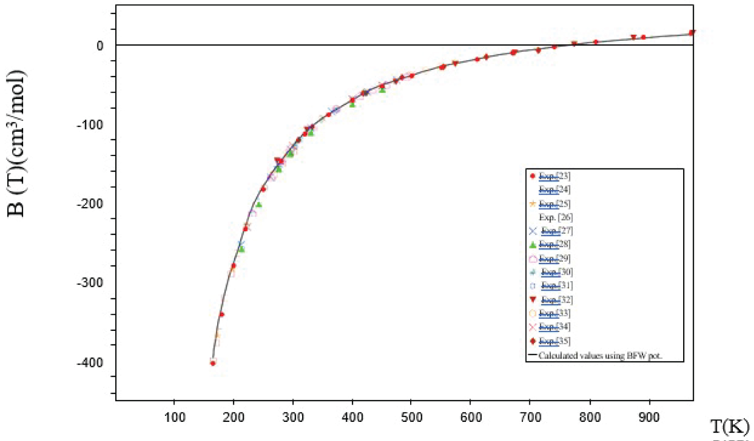
An effective means for checking the validity of the different potential parameters can be made using second pressure virial coefficient data [23-35] at different temperatures. The interaction second pressure virial coefficient B at temperature T was calculated classically with the first three quantum corrections from [57]:

$$B(T)=B_{cl}(T)+\lambda B_{qm,1}(T)+{\lambda }^2{B}_{qm,2}(T)++{\lambda }^3{B}_{qm,3}(T)\left(5\right)$$

Where,

$$B_{cl}(T)=2\pi N_0{\displaystyle \underset{0}{\overset{\infty }{\int }}\left[1-\exp \left[-\frac{V(r)}{k_{B}T}\right]\right]}{r}^{2}dr\left(6\right)$$

With $\lambda ={\hslash }^2/(12m{k}_{B}T)$, $\hslash =h/2\pi$.m and $N_0$ are the atomic mass and Avogadro's number. The first three quantum corrections $B_{qm,1}(T),B_{qm,2}(T)and{B}_{qm,3}(T)$, are given in Ref. [57].

The calculated B₁₂ was compared with the experimental results [23-35] using the present BFW intermolecular potentials. As it may be clearly seen in Figure 1 and Table 1, the interatomic BFW and MTT potentials give the best agreement with the experimental values over a high range of temperatures.

Analysis of traditional transport properties

An additional check on the proposed potential consists of the calculation of the transport properties i.e. viscosity $\eta (T)$, diffusion coefficient D(T), thermal conductivity $\lambda (T)$ and isotopic thermal factor ${\alpha }_{iso}(T)$ at different temperatures T of xenon. These are obtained via the formulae of Monchick, et al. [58] and their comparison to the accurate experimental and theoretical results [36-52] which are clear by calculating the associated values of ${\delta }_j$ as shown in Table 1. The agreements for system under consideration are excellent in the whole temperature range.

Application to the Calculation of Light Scattering Spectra

Principles of CILS spectrum calculations

In a gas of atoms or molecules excited by a laser line of wavelength ${\lambda }_L$, a light scattering spectrum is observable on both sides of the Rayleigh line, the origin of which can be attributed to collision-induced (CI) interactions. By studying this spectrum at different pressures, it is possible to extract its part proportional to the square of the density due to binary interactions [59]. Moreover, the incident laser beam can be polarized parallel (//) or perpendicular $(\perp )$ to the scattering plane. Two binary spectra can therefore be distinguished: The "depolarized" collision-induced light scattering (CILS) spectrum I // (v) and the "polarized" spectrum $I_{{}_{\perp }}(v)$ where n stands for the frequency shift relative to $v_L=c/{\lambda }_L$. In a typical 90° scattering experiment, these two experimental spectra can be expressed in terms of the isotropic^a spectrum $I_0(v)$ and anisotropic spectrum $I_2(v)$

generated, respectively, by the trace $\alpha (r)$ and anisotropy $\beta (r)$ of the CI polarizability tensor of a pair of atoms interacting at a distance r: [1]

$$\left(\begin{array}{c}{I}_{\perp }(v)\\ I_{//}(v)\end{array}\right)=\left(\begin{array}{cc}1& 7/45\\ 0& 2/15\end{array}\right)\left(\begin{array}{c}{I}_0(v)\\ I_2(v)\end{array}\right)$$

The knowledge of the depolarized and isotropic spectra allows therefore to test the models of induced polarizability and intermolecular potential of the studied gas. For a relatively heavy atom such as xenon, a semiclassical approximation with quantum corrections may suffice to calculate its depolarized spectrum $I_{{}_{\perp }}(v)$ and its isotropic spectrum $I_{{}_0}(v)$ at least over the spectral width that has been experimentally explored to date (less than v = 130 cm^-1 in this case [2-5]). Here, we applied the same semi-classical method as the one already successfully used for rare gas mixtures such as Ne-Ar or Kr-Xe [60] or more recently for pure krypton [11]. To summarize what we have described in detail in these papers, we have first calculated the depolarized and isotropic classical spectra $I^{{}^{cl}}(v)$ from the calculation of atomic trajectories for a pair of atoms. For each spectrum, we then distinguished two contributions: That of the pairs of bound or metastable atoms (BM), trapped in the well of the effective interatomic potential (about one third of the depolarized integrated intensity and between 33% and 40% in the isotropic case for xenon at 295 K), and those of the pairs of free atoms (FR) circulating between infinity and the effective potential barrier. At this stage of the calculation, the moments (necessarily even) of a classical spectrum must be equal to the corresponding moments $K_{2n}$ calculated by using the sum rule for n = 0, 1 and 2 [11]:

$$K_{2n}=2k_0{}^{-4}{\displaystyle \underset{0}{\overset{\infty }{\int }}{I}^{cl}}(v){(2\pi v)}^{2n}dv\left(8\right)$$

To obtain the semiclassical spectra of Xenon, we multiplied $I^{cl}(v)$ by a desymmetrization function $D(v)=(1+\delta \Lambda (v))\exp (2\pi \nu {\tau }_0)$, where ${\tau }_0=\hslash /2k_{B}T$ and $\delta \Lambda (v)$ is an even function of quantum origin specific to the studied spectrum. On the one hand, these semiclassical spectra necessarily respect the detailed balance principle, $I(v)=I(-v)\exp (4\pi v{\tau }_0)$. On the other hand, according to our method described in our previous paper [11], the $\delta \Lambda (v)$ function is fitted so that

$$\delta K_{2n}=2k_0^{-4}{\displaystyle \underset{0}{\overset{\infty }{\int }}\delta \Lambda (v)I^{cl}}(v)\cosh \left(2\pi \nu {\tau }_0\right){\left(2\pi \nu \right)}^{2n}dv\left(9\right)$$

Where $\delta K_{2n}$ stands for the Wigner-Kirkwood quantum correction [61] of the classical spectral moment $K_{2n}$. As a final check, the successive semiclassical moments

$$M_n=K_0^{-4}{\displaystyle \underset{-\infty }{\overset{\infty }{\int }}I(v){\left(2\pi \nu \right)}^{2n}}dv\left(10\right)$$

must be close to those deduced from the classical moments, their Wigner-Kirkwood corrections and their dynamical quantum corrections (${\tau }_0^2{K}_{2n}$ divided by 2 or 6) calculated by using the sum rule: [11]

$$\left\{\begin{array}{c}{M}_{2n}\underset{n\ge 0}{=}{K}_{2n}+\delta K_{2n}+\frac{{\tau }_0^2}{2}{K}_{2n+2}\\ M_{2n-1}\underset{n\ge 1}{=}{\tau }_0\left(K_{2n}+\delta K_{{}_{2n}}+\frac{{\tau }_0^2}{6}{K}_{2n+2}\right)\end{array}\right.\left(11\right)$$

In the case of Xenon, the dynamical quantum and Wigner-Kirkwood corrections are very small, almost negligible for $M_{{}_0}$ and M₂ and of the order of a percent for M₄ Furthermore, the moments calculated from the computed spectra match the moments calculated by the sum rule to within 1%.

Depolarized Spectrum: Results and Analysis

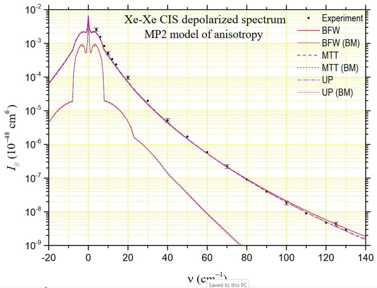
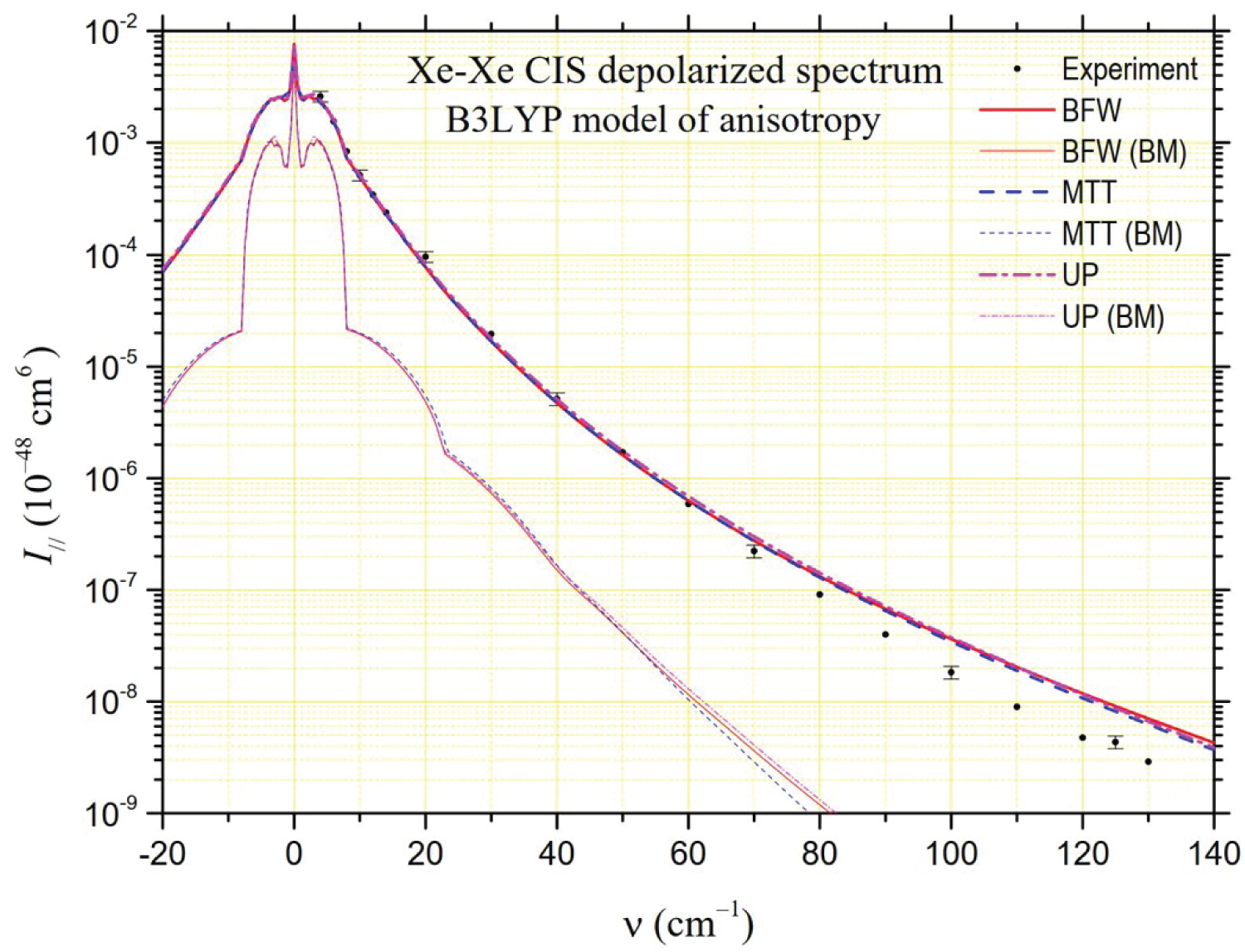
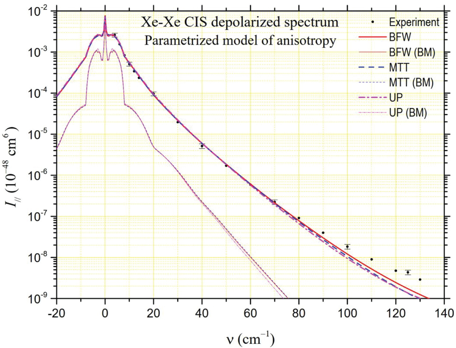
The depolarized spectrum of xenon at 294.5 K is shown in Figure 2, Figure 3 and Figure 4. On these figures, the experimental values determined by Dixneuf, Chrysos and Rachet (DCR) [4] are reported. The experimental values of Zoppi, et al. [3] and of Profitt, Keto and Frommhold (PKF) [2] are not reported since they are very close to the previous ones and can hardly be distinguished from them on a logarithmic scale. In the same figures, theoretical depolarized spectra are reported by using three potentials: The "universal" potential (UP) defined in Ref. [8] and used by DCR, and the BFW and MTT potentials presented in this work. Intensities generated by the MP2 and B3LYP anisotropies calculated ab initio by Maroulis, et al. [6] are presented in Figure 2 and Figure 3, respectively. The UP/MP2 spectrum is very close to the one calculated by DCR using quantum methods, which confirms partly the relevance of our semiclassical method. Nevertheless, our UP/B3LYP intensities diverge by higher values from DCR calculations beyond 100 cm^-1. In Figure 2, compared to the experimental measurements, a lack of intensity is noticeable below 70 cm^-1 for the MP2 model regardless of the potential, while the agreement is satisfactory for higher frequencies. The result is the opposite in Figure 3 for the B3LYP model, which generates intensities close to the experiment at low frequencies but generates too high intensities above 70 cm^-1. In Figure 4, intensities correspond to our analytical model of polarizability, hereafter referred to as the parameterized model (PM),

$\beta (r)=\frac{6{\alpha }_0^2}{r^3}+\left(6{\alpha }_0^3+\frac{\gamma C_6}{3{\alpha }_0}\right)\frac{1}{r^6}+\frac{24{\alpha }_0^{2}C}{r^8}-g_2\exp \left(-\frac{r-\sigma }{r_{21}}-\left(\frac{r-\sigma }{r_{22}}\right)\right)\left(12\right)$

where, ${\alpha }_0=28.44e^{{}^2}{a}_{{}_0}^{{}^2}{E}_{{}_h}^{{}^{-1}}$, $\gamma =8605e^{{}^4}{a}_{{}_0}^{{}^4}{E}_{{}_h}^{{}^{-3}}$ and $C=233.47e^{{}^2}{a}_{{}_0}^{{}^4}{E}_{{}_h}^{{}^{-1}}$ stand for atomic polarizability, hyperpolarizability and quadrupole polarizability, respectively (B3LYP [6]), C₆ = 285.9 au (DOSD [56]) for the dispersion force coefficient, and $\sigma$ = 7.389 bohrs for the xenon diameter. Besides, $g_2$ = 2.159 au, $r_{{}_{21}}$ = 0.655 bohrs and $r_{22}$ = 1.890 bohrs are fitted parameters obtained according the analysis of CILS spectral moments described in Ref. [11]. In this PM case, based on often used empirical models [2,62,63], the agreement with the experiment is very good at low frequencies while a slight deficit in intensity appears at higher frequencies. For MP2 and PM models, the BFW potential generates higher intensities at high frequencies and appears to respond best to the experimental data.

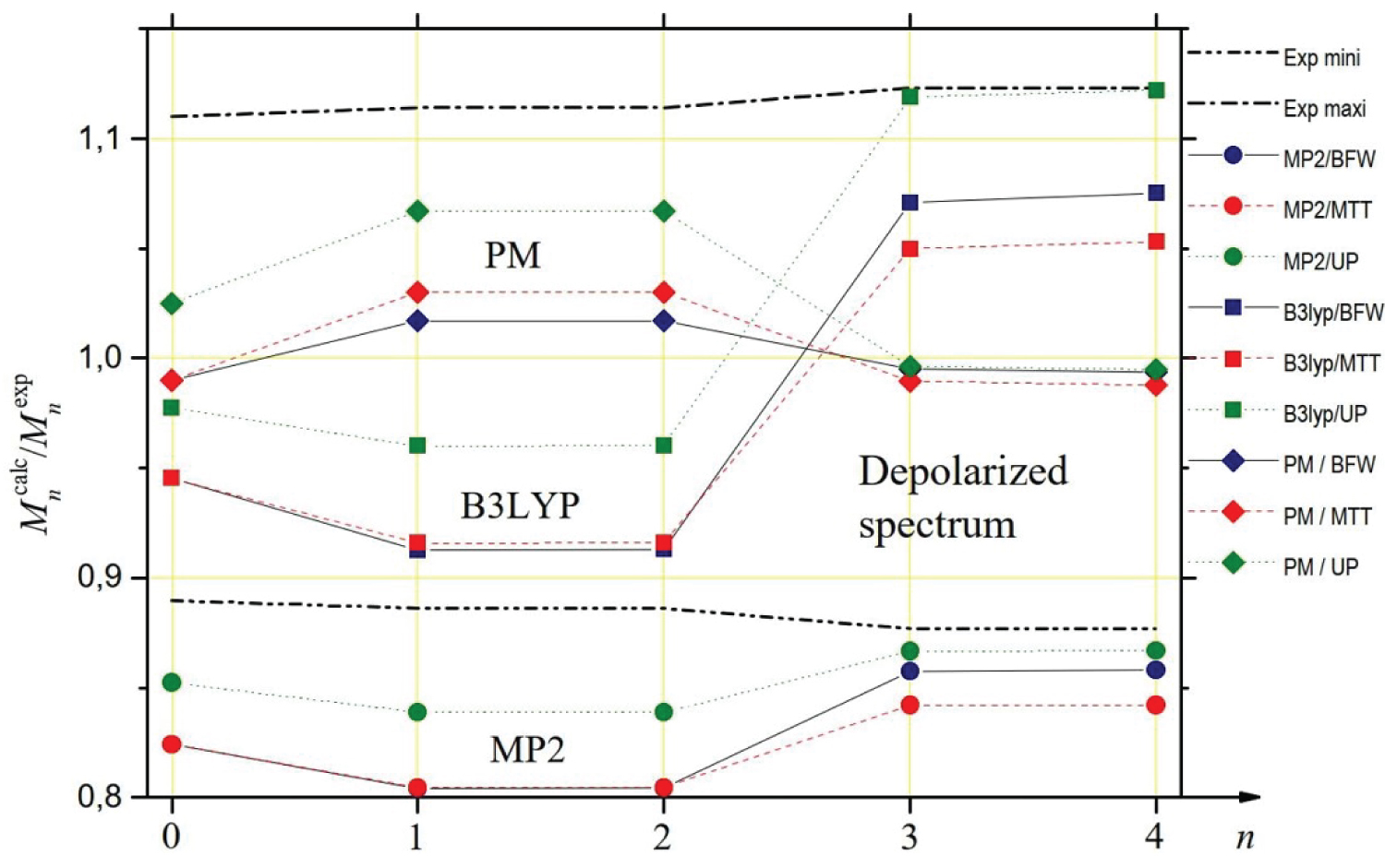
In Table 3, we report the values of the spectral moments $M_n(n=1to4)$ that can be deduced from the theoretical spectra for the three potentials considered (BFW, MTT, UP), two quantum models of polarizability calculated by Maroulis (MP2, B3LYP) [6] and our parametrized model (PM). We also report the values of the moments that can be deduced from DCR experimental data [4]. Since these experimental intensities could only be measured from 4 cm^-1, due to the presence of the Rayleigh line, we had to extrapolate the values of the successive experimental moments in the interval [0, 4] cm^-1. To do this, we based ourselves on the observation that, whatever the polarizability model and the potential considered, the theoretical contribution of this interval is about 53% for M₀, 4.3% for M₁ and M₂, 0.63%_o for M₃ and M₄. Besides in Figure 5, it is possible to visualize the ratios $M_n^{calc}/M_n^{\exp }$ between the successive calculated and experimental spectral moments. We also considered the lower and upper limits of the ratios between theoretical and experimental moments by taking into account the uncertainty bars of the experimental measurements. The MP2 model of anisotropy [6] fails to fall within the limits set by the uncertainty bars because of the too low intensities it generates at low frequencies. The MP2 depolarized intensities are close to experiment beyond 70 cm^-1 but it is not sufficient to get moment values compatible with those inferred from experiment (even for M3 and M₄ because the interval [70, $\infty [c{m}^{-1}$ contributes only about one-fifth of these high-order moments). The spectral moments associated with the B3LYP model are within the uncertainty bars, but with values of M₃ and M₄ close to the upper limit (this time, the frequency range beyond 70 cm^-1 where the values of the B3LYP intensities exceed the experimental intensities contributes 30%). From the analysis of Table 3 and Figure 4, it appears that the PM model is the one that, whatever the chosen potential, is fully compatible with the experimental measurements of the spectral moments. Indeed, this is a logical consequence of the way this analytical model was developed, based on the analysis of spectral moments.

Isotropic Spectrum

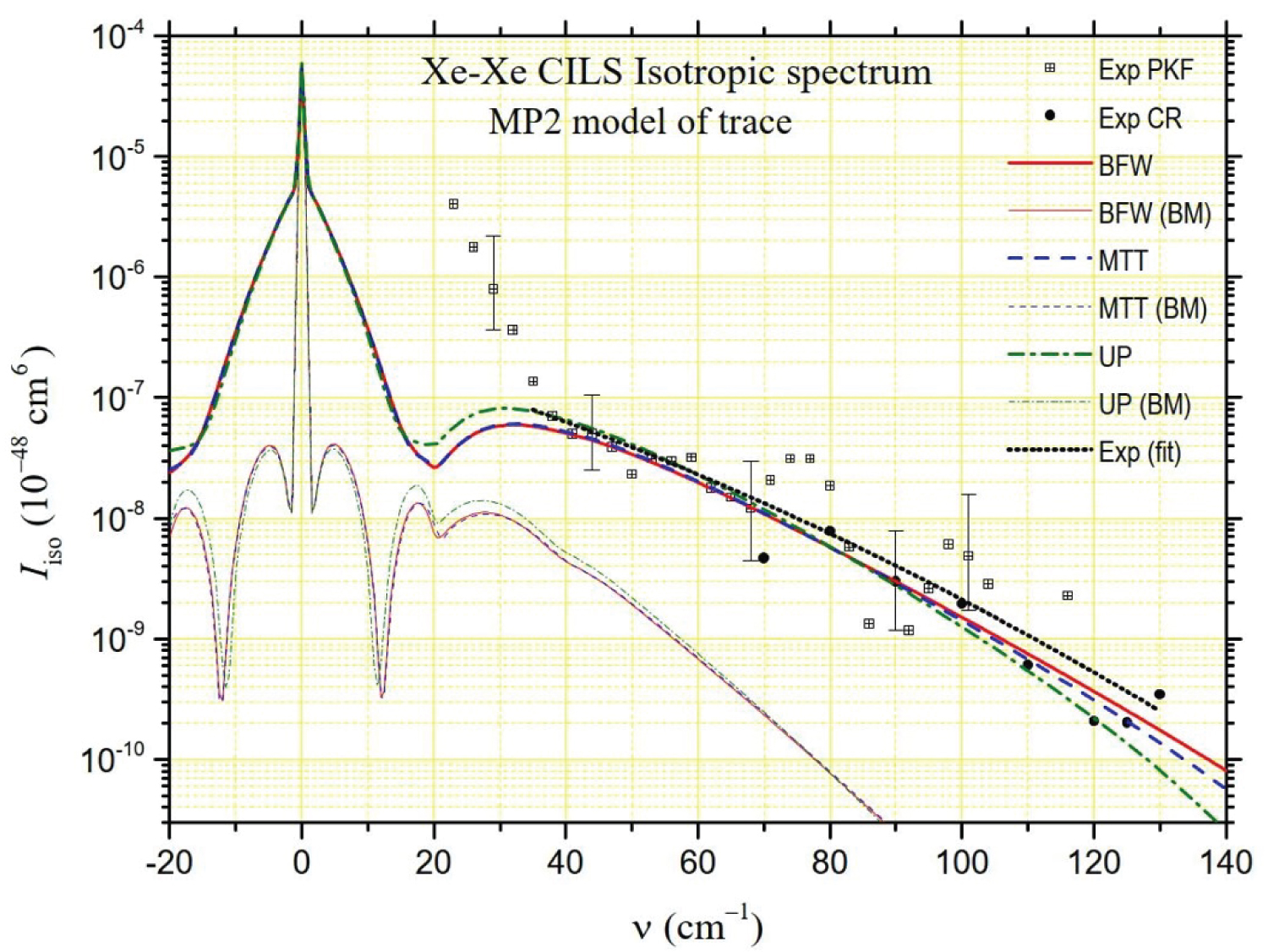
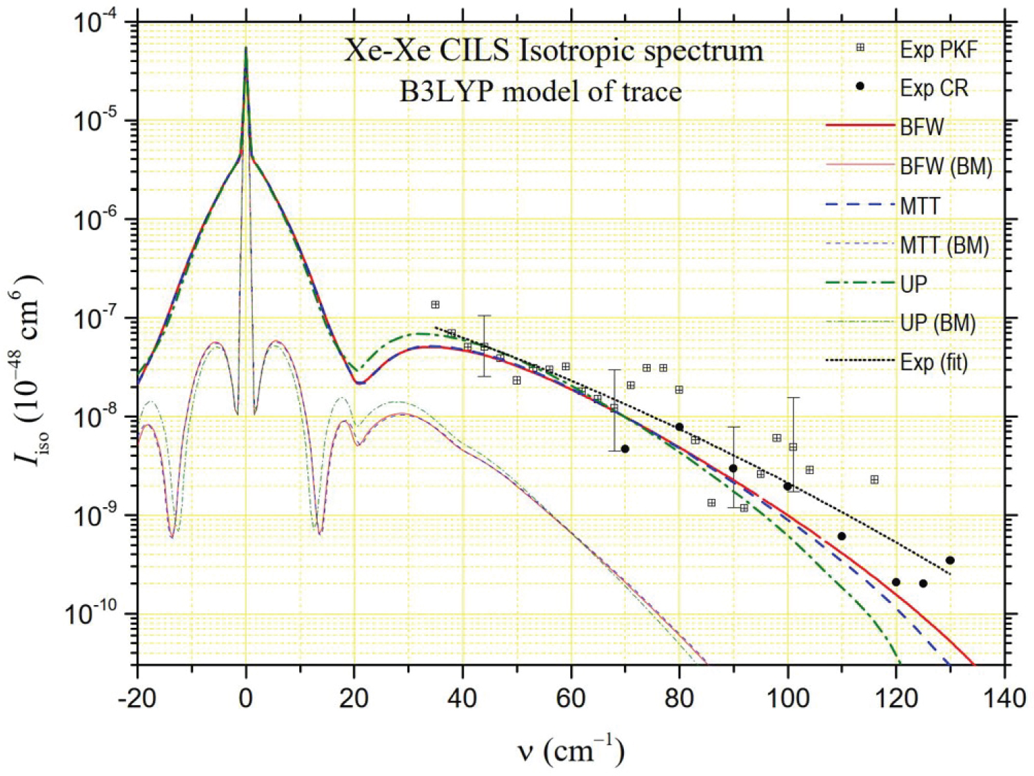
Results and analysis the analysis of the isotropic spectrum is much more delicate. Experimentally, two series of measurements are available, performed by PKF [2] and more recently by Chrysos and Rachet (CR) [5]. Given the uncertainty bars, these series are compatible. However, uncertainties are very large. This is because the spectrum is deduced, according to Eq. (7), from the subtraction of two quantities,

$$I_0(v)=I_{\perp }(v){-}_6^7{I}_{//}(v)\left(13\right)$$

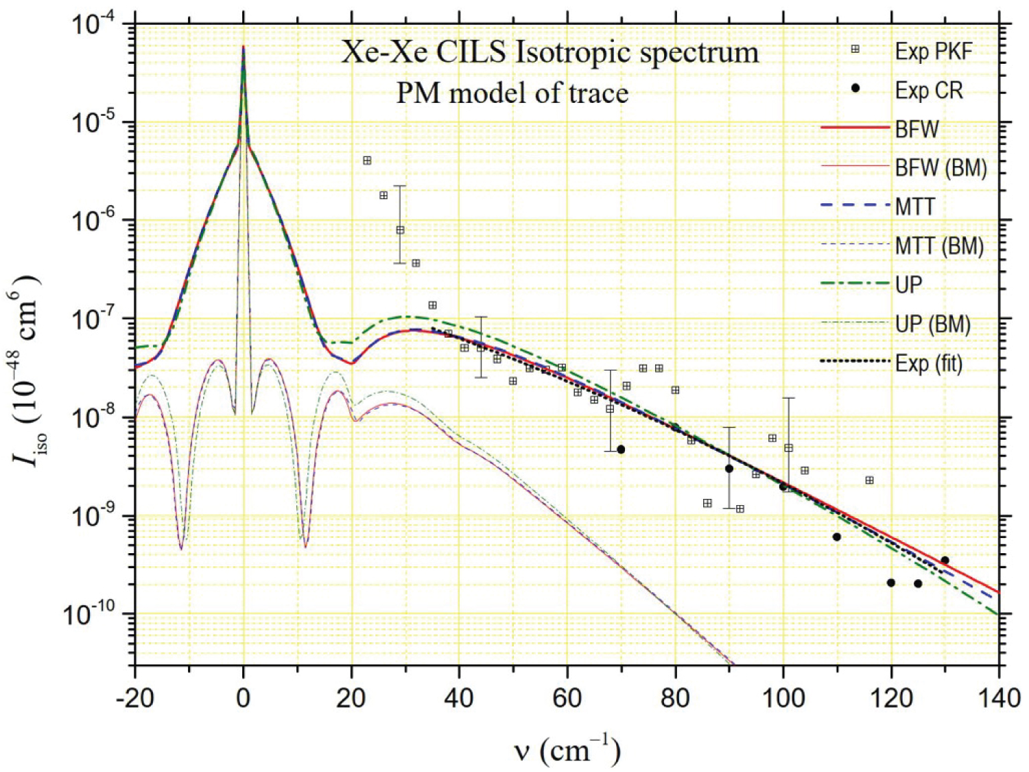
that are generally close together. The isotropic intensities $I_0(v)$ are of the order of a few percent of $I_{\perp }(v)$ at lower frequencies even if they can reach a few tenths at the highest frequencies. Moreover, the presence of the Rayleigh line and its wings makes it particularly difficult to determine $I_{\perp }(v)$ at low frequencies (and also the depolarized spectrum $I_{//}(v)$ at $v\approx 0$). Thus, PKF's isotropic spectrum measurements only start at 23 cm^-1. Even more revealing of the experimental difficulties in extracting the isotropic spectrum from the polarized and depolarized spectra, these of Chrysos and Rachet start at 70 cm^-1. We report both series of intensities in Figure 6, Figure 7 and Figure 8. The experimental spectrum appears to be divided into two parts. Up to about 35 cm^-1, the intensity decreases strongly in an almost exponential way. Beyond, the decrease is less strong while gradually stronger. The large dispersion of the experimental data can be noticed in the latter frequency range, in accordance with the big size of the uncertainty bars. For this reason, using the least squares method, we calculated "average" experimental intensities by degree 2 polynomial fitting of the logarithms of all the experimental intensities (these of PKF and these of CR) from 35 cm^-1 to 130 cm^-1. The "synthesis" curve thus obtained is represented by a black dotted line in Figure 6, Figure 7 and Figure 8. In Figure 6 and Figure 7, we also present the theoretical intensities generated by the MP2 and B3LYP models of trace of Maroulis [6] for the three potentials considered in this work (BFW, MTT, UP [8]). In Figure 8, we present similarly the theoretical isotropic spectrum generated by the PM trace,

$$\alpha (r)=\left(4{\alpha }_0^3+\frac{5\gamma C_6}{9{\alpha }_0}\right)\frac{1}{r^6}+\frac{20{\alpha }_0^{2}C}{r^8}-g_0\exp \left(-\frac{r-\sigma }{r_{01}}-{\left(\frac{r-\sigma }{r_{02}}\right)}^2\right),\left(14\right)$$

Where $g_0$ = 1.275 au, $r_{01}$ = 0.49 bohrs and $r_{02}$ = 2.958 bohrs are fitted parameters deduced from the method presented in Ref [11], as for the PM anisotropy. From the analysis of the figures, it appears that the model that comes closest to the "synthesis" curve is the PM model for MTT or BFW potentials. However, regardless of the potential, both MP2 and B3LYP models are fully consistent with the experimental data in the 35-130 cm^-1 frequency range. Below 35 cm^-1, PKF's measurements need to be confirmed, given the uncertainties in measuring the polarized spectrum at low frequencies. The quasi-exponential growth in intensity as the frequency shift tends to zero is nevertheless found with the MP2, B3LYP and PM models, albeit at lower frequencies.

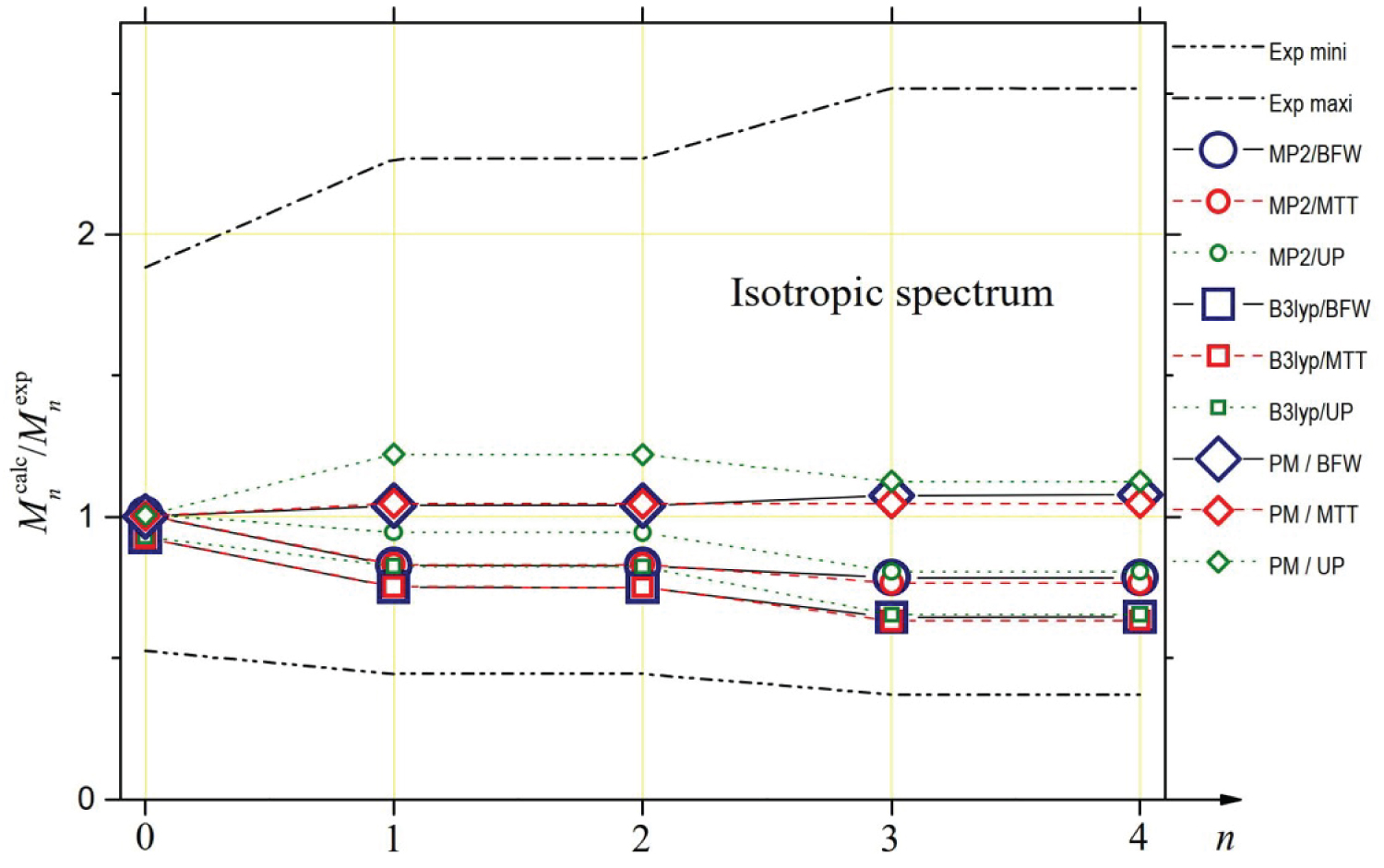
The study of the spectral moments confirms the previous considerations, albeit in a more uncertain way. The spectral range inaccessible to the experiment is much larger than in the case of the depolarized spectrum. The contribution to the spectral moments of the interval [0, 35] cm^-1 cannot be determined from experimental measurements while it is decisive for the value of $M_0$. However, Figure 8 highlights a very good agreement between the isotropic intensities generated by the PM model (and, to a lesser extent, by the MP2 model) for BFW or MTT potentials and the "synthesis" curve of the experimental measurements of PKF and CR beyond 35 cm^-1. This observation led us to hypothesize that it is possible to extrapolate the relative contributions of the interval [0, 35] cm^-1 to experimental moments from the contributions of the same interval for the PM model and both BFW and MTT potentials: $\approx$ 96.6% for $M_0$, $\approx$ 0.22% for $M_1$ and $M_2$, $\approx$ 0.03% for $M_3$ and $M_4$ (MP2 model gives similar results). Based on this assumption, the experimental spectral moments are listed in Table 4 next to the calculated moments for the three models MP2, B3LYP and PM and the three potentials BFW, MTT and UP. The ratios $M_n^{calc}/M_n^{\exp }$ between the successive calculated and experimental spectral moments are given in Figure 9. This figure confirms that the three trace models studied are compatible with the experiment given the very large uncertainty bars. Of course, and this is the effect of the previously described hypothesis for the interval [0, 35] cm^-1, we find $M_0^{calc}$ / $M_0^{\exp }\approx$ 1 for the PM model of trace whatever the potential is, but it is also checked for the MP2 model and to a lesser extent for the B3LYP model. For the higher order moments, to which the interval [0, 35] cm^-1 contributes little, it is the PM model of the trace that appears to be in best agreement with the experimental measurements, both for the BFW potential and the MTT potential.

Conclusion

In this paper, we applied the methods we developed in previous papers [9-11,60] to determine the potential and polarizability of xenon from the available experimental data. The BFW and MTT potentials thus defined and the parametrized model of the anisotropy and trace of the polarizability tensor of Xenon allowed us to calculate its depolarized and isotropic CIS spectra. The comparison of these theoretical spectra with the experimental spectra measured by several groups [2-5] confirms the validity of our approach. In particular in the case of the isotropic CIS spectrum, it is remarkable that the theoretical spectrum deduced from our models coincides quite exactly with a polynomial fit of degree 2 of the logarithms of all experimental intensities in the interval [0, 35] cm^-1. Indeed, both the BFW and MTT potentials and the trace and anisotropy analytical models (PM) presented in this work are able to account for the available experiments.

References

1. Frommhold L (1981) Collision-induced scattering of light and the diatom polarizabilities. Adv Chem Phys 46: 1.
2. Proffitt MH, Keto JW, Frommhold L (1981) Can J Phys 59: 1459.
3. Zoppi M, Moraldi M, Barocchi F, et al. (1981) Chem Phys Lett 83: 294.
4. Dixneuf S, Chrysos M, Rachet F (2009) Anisotropic collision-induced Raman scattering by the Kr-Xe gas mixture. J Chem Phys 131: 074304.
5. Chrysos M, Rachet F (2015) Heavy rare-gas atomic pairs and the “double penalty”issue: Isotropic Raman lineshapes by Kr2, Xe2, and KrXe at room temperature. J Chem Phys 143: 174301.
6. Maroulis G, Haskopoulos A, Xenides D (2004) Chem Phys Lett 396: 59.
7. Van den Biesen JJH, Stockvis FA, van Veen EH, et al. (1980) Physica A (Amsterdam) 100: 375.
8. Koutselos AD, Mason EA, Viehland LA (1990) J Chem Phys 93: 7125.
9. El-Kader MSA, Taher BM (2003) Z Phys Chem 217: 1127.
10. El-Kader MSA, El-Sadek AA, Taher BM, et al. (2011) Mol Phys 109: 1677.
11. Godet JL, El-Kader MSA (2022) Isotropic and anisotropic collision-induced light scattering spectra of krypton gas simultaneously fitted by ground state interatomic potential. J Quant Spectr Rad Transf 288: 108251.
12. Maitland GC, Rigby M, Smith EB, et al. (1981) Intermolecular forces - their origin and determination. Clarendon, Oxford.
13. Maitland GC, Wakeham WA (1978) Mol Phys 35: 1443.
14. Cohen ER, Birnbaum G (1975) J Chem Phys 62: 3807.
15. Sheng X, Zhu H, Zhang Z, et al. (2019) Int J Quant Chem 119: e25800.
16. Xie JC, Kar T, Xie RH (2014) Chem Phys Lett 591: 69.
17. Hellmann R, Jäger B, Bich E (2017) J Chem Phys 147: 034304.
18. Aziz RA, Slaman MJ (1986) Mol Phys 57: 825.
19. Dham AK, Meath WJ, Allnatt AR, et al. (1990) Chem Phys 142: 173.
20. Slavı́ček P, Kalus R, Paška P, et al. (2003) J Chem Phys 119: 2102.
21. Hanni M, Lantto P, Runeberg N, et al. (2004) Chem Phys 121: 5908.
22. Freeman DE, Yoshino K, Tanaka Y (1974) J Chem Phys 61: 4880.
23. Dymond JH, Marsh KN, Wilhoit RC, et al. (2002) Virial coefficients of pure gases and mixtures. Edited by Frenkel M, Marsh KN, Landolt-Bornstein, Heidelberg - Group IV Physical Chemistry, 21, Subvolume A “Virial Coefficients of Pure Gases” Springer-Verlag.
24. Pollard C (1971) Thesis, Univ London, London, England.
25. Brewer J (1967) Technical Report No AFOSR, 67-2795.
26. Hahn R, Schaefer K, Schramm B et al. Phys Chem 78: 287.
27. Schmiedel H, Gehrmann R, Schramm B (1980) Ber Bunsen-Ges Phys Chem 84: 721.
28. Schramm B, Mueller W (1982) Ber Bunsen-Ges Phys Chem 86: 110.
29. Schramm B, Schmiedel H, Gehrmann R, et al. (1977) Ber Bunsen-Ges Phys Chem 81: 316.
30. Michels A, Wassenaar T, Louwerse P (1954) Physica 20: 99.
31. Reeves CG, Whytlaw-Gray R Proc R Soc London, A 232: 173.
32. Whalley E, Lupien Y, Schneider WG (1955) Can J Chem 33: 633.
33. Beattie JA, Barriault RJ, Brierley JS (1951) J Chem Phys 19: 1222.
34. Perez S, Schmiedel H, Schramm B (1980) Z Phys Chem (Munich) 123: 35.
35. Rentschler HP, Schramm B (1977) Ber Bunsenges Phys Chem 81: 319.
36. Clarke AG, Smith EB (1968) J Chem Phys 48: 3988.
37. Dawe RA, Smith EB (1970) J Chem Phys 52: 693.
38. Goldblatt M, Wageman WE (1971) Phys Fluids 14: 1024.
39. May EF, Berg RF and Moldover MR (2007) Int J Thermophys 28: 1085.
40. Lin H, Che J, Zhang JT (2016) Fluid Phase Equilib 418: 198.
41. Vogel E (2016) Int J Thermophys 37: 63.
42. Srivastava BN, Barua AK (1960) J Chem Phys 32: 427.
43. Saxena SC, Davis FE (1971) J Phys E4: 681.
44. Vargaftik NB, Yakush LV (1971) J Eng Phys 21: 1156.
45. Springer GS, Wingeier EW (1973) J Chem Phys 59: 2747.
46. Shashkov AG, Nesterov NA, Sudnik VM (1976) Eng Phys 30: 439.
47. Kestin J, Paul R, Clifford AA et al. (1980) Physica A 100: 349.
48. Assael MJ, Dix M, Lucas A, et al. (1981) J Chem Soc FaradayTrans 177: 439.
49. Le Neindre B, Garrabos Y, Tufeu R (1989) Physica A 156: 512.
50. Visner (1951) In “Proceedings of the American Physical Society,” Phys Rev 82: 291.
51. Amdur I, Schatzki TF (1957) J Chem Phys 27: 1049.
52. Kestin J, Knierim K, Mason EA, et al. (1984) J of Phys and Chem Ref Data 13: 223.
53. Barker JA, Fisher RA, Watts RO (1971) Mol Phys 21: 657.
54. Peng JF, Li P, Ren J, et al. (2011) J At Mol Sci 2: 289.
55. Tang KT, Toennies JP (1984) J Chem Phys 80: 3726.
56. Thakkar AJ, Hetterna H, Wormer PES (1992) J Chem Phys 97: 3252.
57. Bich E, Hellmann R, Vogel E (2008) Mol Phys 106: 1107.
58. Monchick L, Yun KS, Mason EA (1963) J Chem Phys 39: 654.
59. Elliasmine A, Godet JL, Le Duff Y (1997) Mol Phys 90: 147.
60. Godet JL, El-Kader MSA (2019) Collision-induced light scattering (CILS) and collision-induced absorption (CIA) spectra for monatomic rare gas mixtures. J of Quant Spectr Rad Transf 231: 239.
61. Hartye RW, Gray CG, Poll JD et al. (1972) Mol Phys 29: 825.
62. Meinander N, Tabisz GC, Zoppi M (1986) J Chem Phys 84: 3005.
63. El-Sheikh SM, Tabisz GC, Buckingham AD (1999) Chem Phys 247: 407.