The Membranous Labyrinth in vivo from High-Resolution Temporal Bone CT Data

Abstract

Purpose: A prerequisite for the modeling and understanding of the inner ear mechanics needs the accurate created membranous labyrinth. We will present a semi-automated methodology for accurate reconstruction of the membranous labyrinth in the cochlea from high-resolution temporal bone CT data.

Method: We created the new imaging technique which was combined with the segmentation methodology, transparent, Thresholding, and opacity curve algorithms. This technique allowed the simultaneous multiple images creating without any overlapping regions in the inner ear has been developed from temporal bone CT data.

Results: The reconstructed 3D images improved the in vivo cochlear membranous labyrinth geometry to realistically represented physiologic dimensions. These generated membranous structures were in good agreement with the previously published ones, while this approach was the most realistic in terms of the membranous labyrinth in the cochlea.

Conclusions: The precise volume rendering depends on proprietary algorithms so that different results can be obtained, and the images appear qualitatively different. For each anatomical question, a different visualization technique should be used to obtain an optimal result. All researchers can create the in vivo 3D membranous labyrinth in the cochlea in real-time like a retinal camera. This technique will be applied to a cone-beam CT dataset.

Keywords

3D imaging, Volume CT, Otologic Diagnostic Technique, Membranous, labyrinth, Inner Ear, Cochlea

Abbreviations

3D: Three-dimensional; PC: Personal computer; MIP: Maximum intensity projection; VR: Volume rendering; DLP: Dose length product; WW: Window width; WL: Window level; HU: Hounsfield units; CBCT: Cone-beam CT

Introduction

Developments of radiological modalities and analytic techniques of imaging data have resulted in a steady increase in volume and improvement in the accuracy of the inner ear imaging in the cadaver at a level of a light microscope by using micro-CT and micro-MRI [1]. As scientists have workstations or a PC that downloaded an open-source 3D software, they have come to gain the capabilities for the reconstruction and evaluation of 3D post-processing from the volume data. The 3D reconstructed methods such as maximum intensity projection (MIP), surface rendering, and volume rendering (VR) are the most common computer algorithm used to transform axial volume CT or MRI image data into 3D images. Therefore, the bony labyrinth has been popular to reconstruct from CT or MRI data from the 1990s [1-3]. If the soft tissue structures within the osseous labyrinth will be depicted, it will be the image of the membranous labyrinth. In volume rendering (VR) algorithm, high opacity values produce an appearance like surface rendering, which helps display complex 3D relationships clearly. Low opacity value creations can be very useful for seeing a tumor within the lumen [4,5]. It is possible to create an image of the low-density subject behind the high-density subject according to the opacity property. Voxel opacity curve algorithms can be adjusted to render tissues within a certain density range. Thresholding extracts an interesting region by selecting a range of a target tissue voxel value [6,7]. Therefore, by combining these algorithms, the low-density structure of the membranous labyrinth behind the bone density of the osseous labyrinth can be depicted [8]. This study aims to develop and use the volume rendering (VR) algorithms for allowing in vivo 3D transparent visualization of the membranous labyrinth in the cochlea from high-resolution CT data sets, and to evaluate by comparing the created 3D microanatomical images with the previous histological ones.

Materials and Methods

Participants

Participants imaging data from 10 volunteers (5 men and 5 women, mean age 41.7, range of age: 16-62) who visited for their regular medical checkups and wished to examine the head and temporal bone regions were obtained. These participants had no known affliction of the temporal bone and no hearing problem, or other systems related to auditory and vestibular systems and normal findings on both CT exams and physical exam by their checkups. This retrospective study was conducted under the approval of the clinic institutional review board, and the written informed consents were obtained from all participants.

CT protocol

All examinations were performed with the spiral CT scanner (ProSpeed AI; General Electric Systems (GE), Milwaukee, Wis., USA) by using an axial technique with 120 kV, 60-120 mA, and 60 seconds scanning time. The section thickness was 1 mm and an interval of 0.5 mm overlapping. A pitch was 1.0. The axial images were reconstructed with a high-resolution bone algorithm in steps of 0.5 mm, and a field of view (FOV) of 96 × 96 mm by using a 512 × 512 matrix. The dose length product (DLP) was recorded on the CT monitor by the GE medical software. The DLP ranged from 40 mGy/cm to 55 mGy/cm.

Volume rendering (VR)

Most VR techniques will be divided into two types [4-7]. One is thresholding or surface-based methods. The other is percentage- or transparent volume-based techniques. Certain properties (opacity, color, shading, brightness) are assigned to each voxel value. The most important property is opacity or attenuation, which enables the user to hide certain objects or make them transparent. Thresholding extracts a region of interest by selecting a range of voxel values that presents a specific tissue or anatomical feature. Voxel opacity curve algorithms can be adjusted to render tissues within a certain density range. In this study, the new algorithms are made from a thresholding method with a transparent volume-based technology under voxel opacity curve algorithms. Therefore, it is necessary to choose which type of a voxel opacity curve algorithm and to set each parameter beforehand for VR imaging. Setting an opacity value is an important factor in creating VR images [8].

Opacity value

Opacity values are determined to define the relative transparency of each material. High opacity values are determined to define the relative transparency of each material. High opacity values produce an appearance like surface rendering, which helps display complex 3D relationships clearly. Low opacity value creations can be very useful for seeing a subject within the lumen [4-8]. Hence, it is possible to observe the low density (high opacity) subject behind the high density (low opacity) subject according to the property of opacity. As for as the cochlea is concerned, by assigning a low density (high opacity) to the soft tissue and a high density (low opacity) to the cochlea, the soft tissue becomes clearly visible among its semi-transparent surroundings of the osseous cochlea. Therefore, the opacity value is defined by the ratio of the CT values between the two subjects [8].

That is, the following equation holds:

$$\alpha =\frac{\beta }{\gamma }\times 100$$

Where α is the opacity value, β is the low CT density value (cochlear soft tissue), and γ is the high CT density value (cochlea).

Select the opacity curve algorithm

A voxel opacity curve algorithm can be adjusted to render tissues within a certain density range. There are three opacity curve algorithms to reconstruct 3D images of the membranous labyrinth in the cochlea as follows:

1. Upward opacity curve algorithm

As the structures over the high threshold value will show a constant high opacity value, under the lower threshold value is 0% opacity value. Thus, it may be used to display bright structures such as bone or vessels in CT data sets [6]. That is, this opacity curve is suitable to delineate the soft tissue structures on the bony labyrinth.

2. Trapezoid opacity curve algorithm

This opacity curve is used to display structures with voxel values within the defined range [7]. This is suitable for the surface structure of the cochlear membranous labyrinth.

3. Downward opacity curve algorithm

In the case of this opacity curve type, it is opposite to an upward opacity curve type. This opacity curve type can be used to display dark structures such as airways, or vessels in black blood MRA technique [9]. It can also be used with a cut plane to display the lumen of a vessel as etched in the plane. This means that lower CT value organs are distinguished from higher CT value subjects. So, this opacity curve is suitable for fibrotic structures in the cochlear membranous labyrinth.

Color shading mode algorithm

When the color shading method is used to create images, the image is shaded based on the orientation of the surfaces in the voxels that contribute to a given pixel and colored according to the value of these voxels [4-8]. Color shading is surface shading, and it can be seen in the final relationship that basing the opacity functions in the color space effectively revealed structures within volumes.

Applying colors algorithm

There are two techniques to create 3D images by applying color methods as follows:

1. Non-merged 3D image

When a non-merged image is colored, everything in it takes on the same color as Figure 1, Figure 2 and Figure 3. To do this, select the image to be colored, then chose the desired color. The coloring of a non-merged image is typically done in preparation for a 3D merging operation. This makes distinguishing the merge objects easier.

2. Merged 3D image

When the coloring is applied to a merged 3D view, each merged 3D model can be colored independently of the others.

Simple segmentation algorithm

As the target organ data existed in the inner ear, roughly simple segmentation of the temporal bone is required using a front cut method [8].

Parameter Setting

Threshold value

To define the optimal threshold CT value to create 3D images of the membranous labyrinth in the cochlea, the CT values within the edge of the cochlea and the vestibule, and the modiolus were measured using 0.5-mm-thick axial HR-CT image slices at the level through the oval window, the cochlea, and the vestibule. All measurements were carried out using the CT workstation (Advantage version 2.0; GE Medical Systems, Milwaukee, Wis). The imaging condition was as follows; WW was 2000HU, and WL was 200HU. Pixel-level analysis of the DICOM viewer yields actual CT values of them. The results were shown in Table 1.

Statistical analysis

Normality of distribution was tested using the Graphical methods. The goodness of fit test for normality was evaluated by Chi-square statistics. Data were analyzed statistical software available through Microsoft Excel 2013 (Microsoft Corporation Redmond, Washington).

Define threshold value

The statistical analysis revealed that the results were suitable for a normal distribution. These results showed that the cochlea CT values were about through 280 to 380 HU, of the modiolus was about through 230 to 280 HU, and of the vestibule were about through 120 to 200 HU. The cochlear duct CT value was the soft tissues within the fluid components in the cochlea. By subtracting the modiolus value from the cochlear value, the approximate cochlear duct value could be obtained. The calculated value was in the range of about 70 to 140 HU, and the average was 105 HU. To know the state of the vestibule together, the highest value of the vestibule was taken as the high threshold value. From the anatomical components, the medullary sheath contained fat. That is, the low absorption value was defined as a fat value of -100 HU, and the high absorption value was 200 HU of the vestibule.

Opacity value

The opacity value was set to the average of 40%.

Brightness value

The brightness value was defined as the constant value of 100%.

Postprocessing

After transferring the image to the CT workstation (GE Medical Systems, Milwaukee, Wis., USA), 3D visualization based on interactive direct volume rendering was made using GE Advantage Navigator software. The direct volume rendering considers some of the image data, so roughly simple explicit segmentation prior to the visualization process was required using a front cut method. The display field of view (DFOV) was 16-32 × 16-32 mm. As a result of this software, both color and opacity values were adjusted interactivity to delineate all structures related to the membranous labyrinth in real-time under the threshold value. After an appropriate setting, the front cut for optimal delineation of the objective structures was defined on axial, coronal, and sagittal projection, the color and opacity table could be stored and used for further studies [10]. Owing to the simple acceleration of the visualization process, the whole procedure was performed in less than 1 minute. The software allowed both distance measurements and volume directly within the 3D scene. This software was almost the same as the open-source Image J software (available at https://imagej.nih.gov/ij/download.html) or Osiri X Lite software (available at http://https://www.osirix-viewer.com) [11].

Quantitative Image Analysis based on the Results of the Previous Literatures

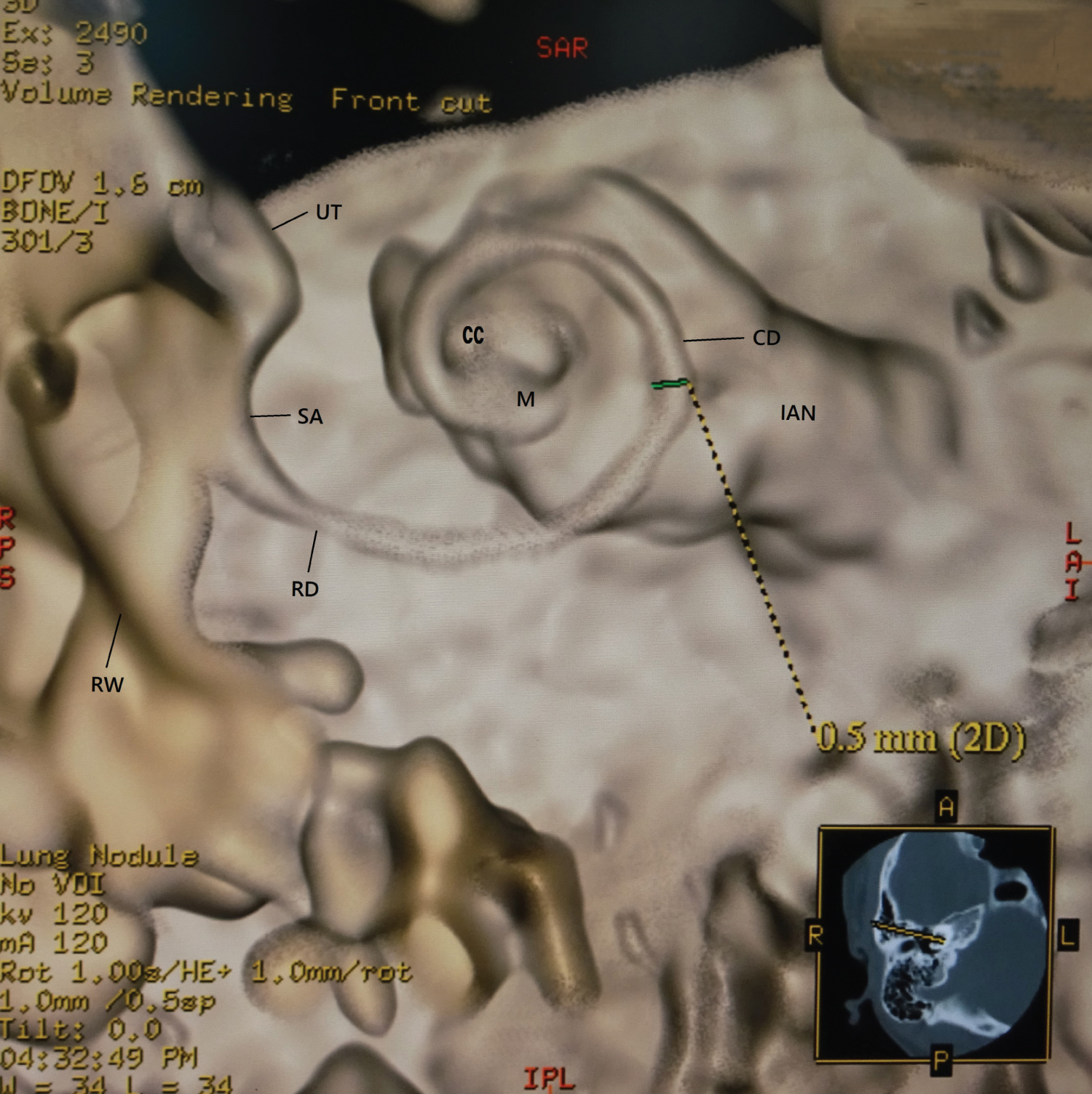
To ascertain whether the 3D created images were consistent with anatomical findings, the cochlear duct width was measured at the position as shown in Figure 2 and compared with the results of the previous histological literatures. The result of the cochlear duct width was 0.40 to 0.60 mm, and then a mean ± SD value was 0.50 ± 0.08 mm. According to the previous literatures, Retzius reported as follows; the height of the lateral wall was from 0.59 to 0.3 mm, the width of the spiral limbus was from 0.22 to 0.23 mm, and the width of the basilar membrane was from 0.21 to 0.36 mm [12]. Wever and Laurence reported that the width of the basilar membrane was between 0.498 to 0.80 mm [13]. That is, the height of the lateral wall was about 0.50 mm, and the width of the floor was about between 0.40 to 0.60 mm. The difference between the results of previous literatures and of this study was assessed for significance by Microsoft Excel 2013using a Wilcoxon rank sum test. A p value of < 0.05 was regarded as significant.

Results

Volume rendering parameters

The threshold value was -100 to 200 HU, the opacity value was 40%, and the brightness value was 100%.

Modeling

The different 3D membranous microanatomical images were created by three different voxel opacity curve algorithms with a merged or non-merged colored technique. The quite different 3D images were made from the different opacity curve algorithm, though Figure 1 and Figure 2 were created from the same direction of the same subject. These created images were the same as that of the published anatomical books and the previous literatures [12-17].

The relation between the created image and the algorithm was as follows:

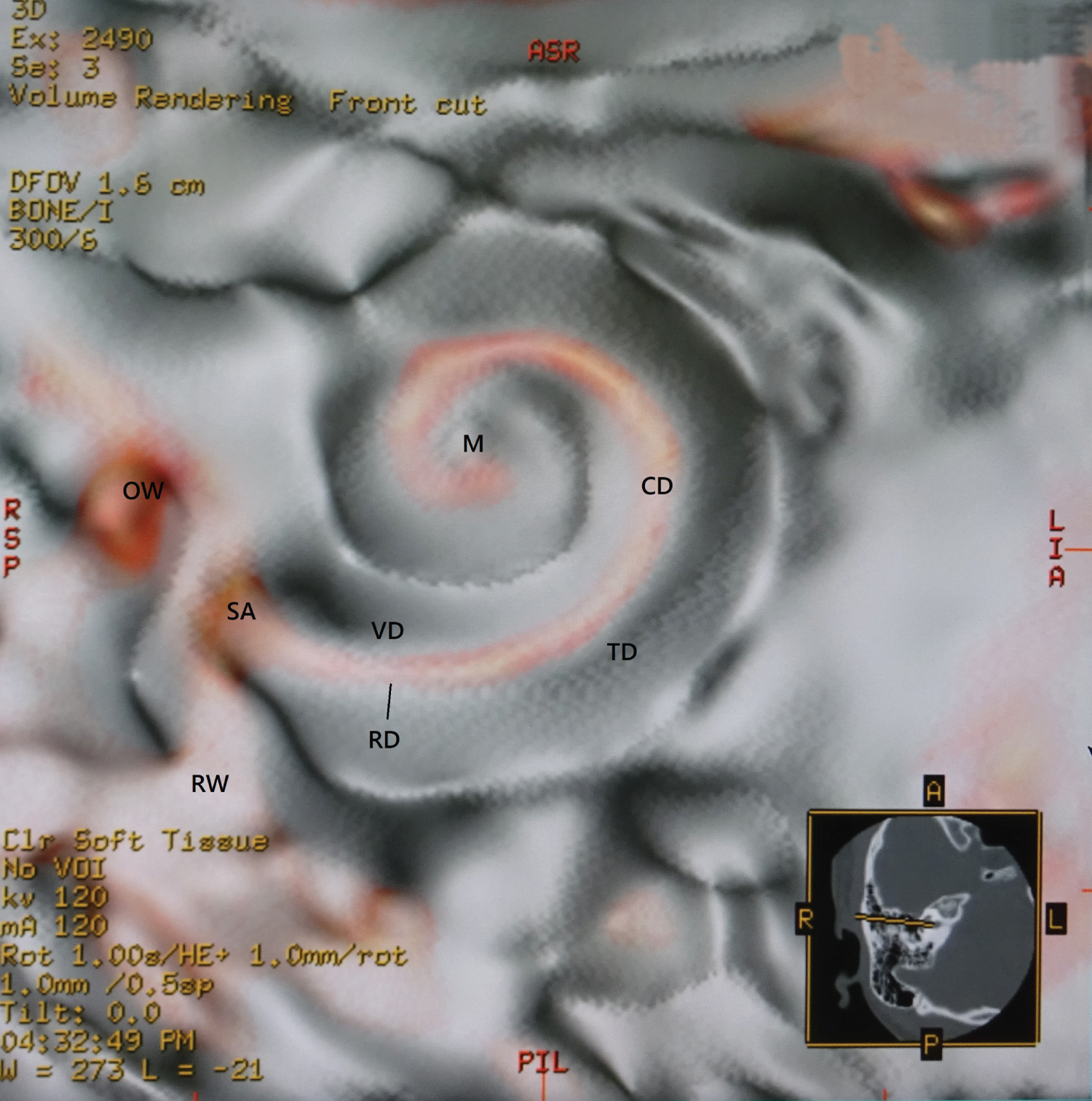
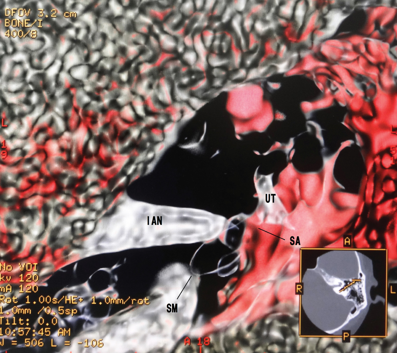
1. An upward opacity curve with a merged color algorithm made the soft tissues of the membranous cochlea on the bone (Figure 1).

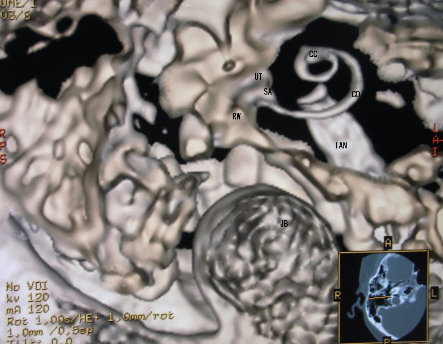
2. A trapezoid opacity curve with a non-merged colored algorithm made surface imaging of the cochlear membranous labyrinth (Figure 2 and Figure 3).

3. A trapezoid opacity curve with a merged colored algorithm created the transparent membranous labyrinth in the cochlea (Figure 4).

4. A downward opacity curve with a merged colored algorithm reconstructed the fibrotic minute structures in the cochlear membranous labyrinth (Figure 5).

Quantitative image analysis

The measured result in the 3D created membranous cochlear duct ranged from 0.40 to 0.60 mm. A significant correlation in comparison with the results of the previous literatures was found p = 0.0048.

Discussion

This study aimed to investigate the non-invasive 3D imaging method of the membranous labyrinth in the cochlea. According to this study, the precise volume rendering depends on proprietary algorithms so that different results can be obtained, and the images appear qualitatively different. For each anatomical question of the membranous labyrinth, a different visualization technique should be used to obtain an optimal result. And, the measured result of the width of the cochlear duct in this study was nearly the same as the histological measurement values in the previous literatures [12,13].

These created membranous cochlea images are similar to the previous histological ones [12-17]. Figure 1 is like removing the lid of the cochlea and looks like the whole soft tissue with the osseous lamina. The cochlear soft tissues are a spring duct between the tympanic duct and the vestibular duct. Figure 2 shows that the cochlear duct is winding along the modiolus, and the shape of the modiolus shows the conical axis. In Figure 3, the cochlear duct has a shape of a triangular spiral tube, and the end of the duct showed like a snakehead is a cupular cecum, and the saccule shows an egg shape from this view. Figure 4 is the anterior cochlear cut image. This image shows that the cochlear duct is a spiral duct and a triangular shape in the cross-section. The duct is suspended between the osseous spiral lamina of the modiolus. The spiral membrane is located within the cochlear duct. The spiral ganglion is situated along the modiolus. Figure 5 represents that the spiral membrane is a spiral winding within the cochlear duct. The diameter of the cochlear duct in Figure 2 and Figure 3 is wider than that of this spiral membrane. The width of a spiral winding becomes wider from the base through the apex. This image is similar to the histological one of the organs of Corti, et al. [16]. Therefore, it is possible to observe the status of the membranous cochlea in real-time without using harmful procedures.

The problem of resolution

The resolution of 3D images is primarily determined by the resolution of the original acquisition images and the inter-slice distance. Although the pixel size of the original 2D image is large, the voxel size of the reconstructed display 3D image is smaller in the practical 3D image. This cause will be based on an algorithm of 3D configuration [18]. It is not possible to identify details within the exam with dimensions in the order of or less than the inter-slice distance with any degree of reliability. Therefore, at all times, it remains the responsibility of the scientist to determine whether the inter-slice distance used for a particular exam is acceptable. Despite the intra-slice distance is 0.5 mm in this study, the created 3D microanatomical images are in good agreement with the previously published ones. However, the more the amount of accurate thin-section 2D data, the more accurate 3D reconstructed images will be created.

The problem of threshold value adapted to any CT or a cone-beam CT

It is defined that the threshold value is obtained from the CT of this study. Therefore, this value cannot be immediately adapted to any CT. However, this defined threshold value will be referred to when setting a threshold value with different CT machines. When these algorithms will be applied for a cone-beam CT (CBCT), we must convert a gray scale value to a Hounsfield unit value. Some studies have shown a strong linear relationship between Hounsfield units (HU) and gray scale [19,20]. Gray scale is different from HU due to higher noise levels, more scattered radiation, high heel effect, and beam hardening artifacts [21,22]. However, we can adapt the rough converted HU obtained from gray scale. Therefore, we believe that this method can also be used for a cone-beam CT (CBCT).

Conclusions

The new interactive transparent volume rendering algorithm is created in combination with thresholding, opacity curve, and transparent algorithms. This new technique allows simultaneous multiple images creating without any overlapping regions in the inner ear, and all scientists can use it easily. Hence, this technique can study the cochlear membranous labyrinth in real-time like a retinal camera. And this technique will be applied to cone-beam CT (CBCT) data.

Compliance with Ethical Standards

Guarantor

The scientific guarantors of this publication are HT and ST. HT and ST contributed equally to this work. HT wrote the final manuscript.

Conflict of interest

We declare no relationship with any companies, whose products or services may be related the subject matter of the article.

Funding

We state that this work has not received any funding.

Statistics and biometry

No complex statistical methods were necessary for this paper.

Informed consent

Written informed consent was obtained from all individual participants in this study.

Ethical approval

All procedures performed in studies involving human participants were accorded with the Ethics Committee of our clinic, and with the 1964 Helsinki Declaration and its later amendments or comparable ethical standards. Institutional Review Board approval was obtained.

Methodology

Retrospective; experimental, performed at one institution.

Preprint

Tanioka H. The Membranous Labyrinth in vivo from high-resolution Temporal CT data.bioRxiv 2018: doi: https://doi.org/10.1101/318030

References

1. Lane JI, Witte RJ (2010) The temporal bone: An imaging atlas. Springer, New York, USA.
2. Tanioka H, Shirakawa T, Machida T, et al. (1991) Three-dimensional reconstructed MR imaging of the inner ear. Radiology 178: 141-144.
3. Fatterpekar GM, Doshi AH, Dugar D, et al. (2006) Role of 3D CT in the evaluation of the temporal bone. Radio Graphics 26: S117-S132.
4. Gelder AV, Kim K (1996) Direct volume rendering with shading via three dimensional textures. In proceeding of 1996 Symposium on Volume Visualization, San Francisco, CA, USA, P: 23-30.
5. Kniss J, Premoze S, Hansen C, et al. (2002) Interactive translucent volume rendering and procedural modeling. IEEE Computer Society, Washington DC, USA, P: 109-116.
6. Heath DG, Soyer PA, Kuszyk BS, et al. (1999) Three-dimensional volume rendering of spiral CT data: Theory and method. Radio Graphics 19: 745-764.
7. Fishman EK, Ney DR, Heath DG, et al. (2006) Volume rendering versus maximum intensity projection in CT angiography: What works best, when, and why. Radio Graphics 26: 905-922.
8. Tanioka H, Tanioka S, Kaga K (2020) Vestibular aging process from 3D physiological imaging of the membranous labyrinth. Sci Rep 10: 9618.
9. Edelman RR, Mattle HP, Wallner B, et al. (1990) Extracranial carotid arteries: Evaluation with "blackblood" MR angiography. Radiology 177: 45-50.
10. Nakao M, Watanabe T, Kuroda T, et al. (2005) Interactive 3D regionextraction of volume data using deformable boundary object. Stud Health Technol Inform 111: 349-352.
11. Amato AC (2016) Surface Length 3D: An OsiriX plugin for measuring length over surfaces. J Vasc Bras 15: 308-311.
12. Retzius G (1884) Das Gehororgan der Wirbeltiere. Morphologisch-histologischeStudien. II. Das Gehororgen der Vogel und der der Sӓugetiere. Stockholm, Denmark: Samson & Wallin, Stockholm.
13. Wever EG, Lawrence M (1954) Physiological acoustics. Princeton University Press, New Jersey, USA.
14. (1989) Human temporal bone research workshop report. Ann Otol Rhinol Laryngol 98: 143.
15. Water TR (2012) Historical aspects of inner ear anatomy and biology that underlie the design of hearing and balance prosthetic devices. Anat Rec 295: 1741-1759.
16. Nomura Y (2006) Morphology in otology. Chugai Iguku, Tokyo, Japan.
17. Toyoda S, Shiraki N, Yamada S, et al. (2015) Morphogenesis of the inner ear at different stages of normal human development. Anat Rec 298: 2081-2090.
18. Lorensen WE, Cline HE (1987) Marching cubes: A high resolution 3D surface reconstruction algorithm. ACM Computer Graphics 21: 163-169.
19. Oliveira ML, Tosoni GM, Lindsey DH, et al. (2014) Assessment of CT numbers in limited and medium field-of-view scans taken using Accuitomo 170 and Veraviewepocs 3De cone-beam computed tomography scanners. Imaging Sci Dent 44: 279-285.
20. Razi T, Emamverdizadeh P, Nilavar N, et al. (2019) Comparison of the Hounsfield unit in CT scan with the graylevel in cone-beam CT. J Dent Res Dent Clin Dent Prospects 13: 177-182.
21. Valiyaparambil JV, Yamany I, Ortiz D, et al. (2012) Bone quality evaluation: Comparison of cone beam computed tomography and subjective surgical assessment. Int J Oral Maxillofac Implants 27: 1271-1277.
22. Parsa A, Ibrahim N, Hassan B, et al. (2012) Reliability of voxel values in computed tomography for preoperative implant planning assessment. Int J Oral Maxillofac Implants 27: 1438-1442.